Avishek Pal - Practical Time Series Analysis: Master Time Series Data Processing, Visualization, and Modeling using Python

>

BIRMINGHAM - MUMBAI

The zero-mean models have a constant mean and constant variance and shows no predictable trends or seasonality. Observations from a zero mean model are assumed to be independent and identically distributed (iid) and represent the random noise around a fixed mean, which has been deducted from the time series as a constant term.

Let us consider that X1, X2, ... ,Xn represent the random variables corresponding to n observations of a zero mean model. If x1, x2, ... ,xn are n observations from the zero mean time series, then the joint distribution of the observations is given as a product of probability mass function for every time index as follows:

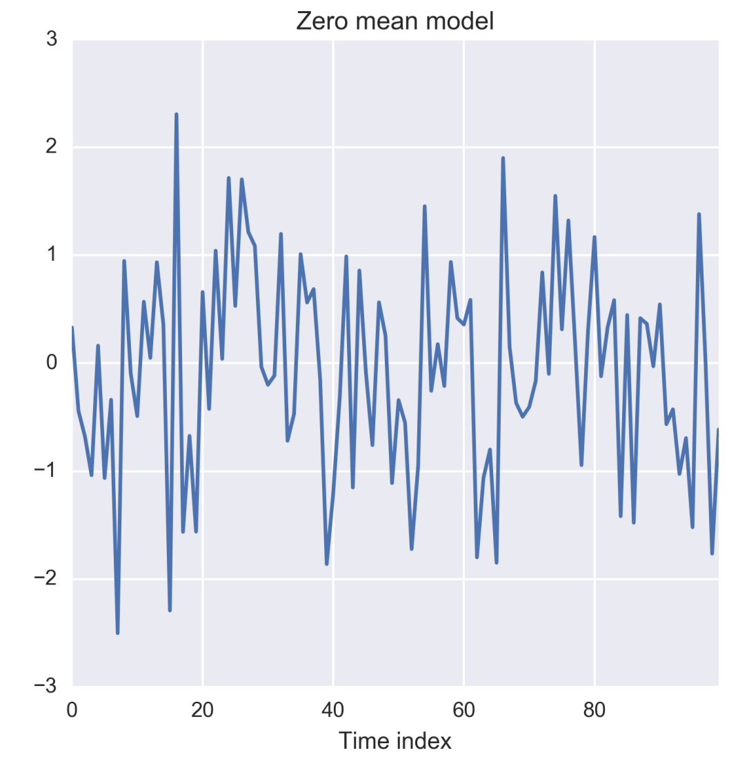
Most commonly f(Xt = xt) is modeled by a normal distribution of mean zero and variance 2, which is assumed to be the irreducible error of the model and hence treated as a random noise. The following figure shows a zero-mean series of normally distributed random noise of unit variance:

The preceding plot is generated by the following code:

The zero mean with constant variance represents a random noise that can assume infinitely possible real values and is suited for representing irregular variations in the time series of a continuous variable. However in many cases, the observable state of the system or process might be discrete in nature and confined to a finite number of possible values s1,s2, ... , sm. In such cases, the observed variable (X) is assumed to obey the multinomial distribution, P(X = s1 )= p1, P(X = s2 ) = p2,,P(X = sm) = pm such that p1 + p2 + ... + pm = 1. Such a time series is a discrete stochastic process.

Multiple throws a dice over time is an example of a discrete stochastic process with six possible outcomes for any throw. A simpler discrete stochastic process is a binary process such as tossing a coin such as only two outcomes namely head and tail. The following figure shows 100 runs from a simulated process of throwing a biased dice for which probability of turning up an even face is higher than that of showing an odd face. Note the higher number of occurrences of even faces, on an average, compared to the number of occurrences of odd faces.

This section describes Convolutional Neural Networks (CNNs) that are primarily applied to develop supervised and unsupervised models when the input data are images. In general, two-dimensional (2D) convolutions are applied to images but one-dimensional (1D) convolutions can be used on a sequential input to capture time dependencies. This approach is explored in this section to develop time series forecasting models.

Seasonality manifests as repetitive and period variations in a time series. In most cases, exploratory data analysis reveals the presence of seasonality. Let us revisit the de-trended time series of the CO2 concentrations. Though the de-trended line series has constant mean and constant variance, it systematically departs from the trend model in a predictable fashion.

Seasonality is manifested as periodic deviations such as those seen in the de-trended observations of CO2 emissions. Peaks and troughs in the monthly sales volume of seasonal goods such as Christmas gifts or seasonal clothing is another example of a time series with seasonality.

A practical technique of determining seasonality is through exploratory data analysis through the following plots:

• Run sequence plot
• Seasonal sub series plot
• Multiple box plots

As you have chosen to read this book, we think that you might have a working knowledge of Python-if not, a hands-on expert who happens to live and breathe Python. In case you have a fair knowledge of Python at the least, you may choose to skip this appendix. If you are new to Python or looking for how to get started with the programming language, reading this appendix will help you get through the initial hurdles. It would also get you what you need to enjoy this book's chapters. So, without further ado, let's jump in!

Python is a general-purpose, high-level, and interpreted programming language, which appeared in 1991. Its creator, Guido van Rossum, started writing the interpretation of the language over the Christmas of 1989 and named the language after one of his favorite TV shows-Monty Python's Flying Circus.

Python emphasizes code readability through whitespace indentation to delimit code blocks rather than curly brackets, which are famously used in C, C++, and Java. Another powerful feature of Python is its succinctness, which allows programmers to express concepts in lines of code fewer than in C, C++, and Java. For example, the use of lambda functions as a quick and effective way of declaring functions in just one line is a favorite among Python developers. (Don't worry; we will get into what a lambda function is later.) Other than these, Python supports dynamic type binding and automatically handles memory for you. Besides, Python interpreters are available for all major operating systems. CPython is the most popular open source implementation of the interpreter. Moreover, Python is supported by hundreds of packages of wide-ranging functionalities such as web development, GUI building, advanced memory management, file handling for diverse file formats, scientific and numeric computing, image processing, machine learning, deep learning, big data, and many others. PyPI is the official repository of Python packages and almost all well-known packages are available there. The link to PyPI's website is https://pypi.python.org/pypi . However, we do not have to download packages from this website before installing. There are command line (CL) tools that do the job for us. These tools are available once a basic version of the language is installed. Moreover, these CL tools take a lot of work from us by ensuring that the requested package is compatible with the current version of Python and that the dependencies are already installed or need to be installed.

This appendix covers the following topics:

• Installation
• Basic data types
• Keywords, control statements, and functions
• Iterators and generators
• Classes and objects

The purpose of time series analysis is to develop a mathematical model that can explain the observed behavior of a time series and possibly forecast the future state of the series. The chosen model should be able to account for one or more of the internal structures that might be present. To this end, we will give an overview of the following general models that are often used as building blocks of time series analysis: