• Complain

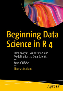
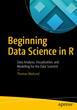
Thomas Mailund [Thomas Mailund] - Beginning Data Science in R: Data Analysis, Visualization, and Modelling for the Data Scientist

Here you can read online Thomas Mailund [Thomas Mailund] - Beginning Data Science in R: Data Analysis, Visualization, and Modelling for the Data Scientist full text of the book (entire story) in english for free. Download pdf and epub, get meaning, cover and reviews about this ebook. year: 2017, publisher: Apress, genre: Computer. Description of the work, (preface) as well as reviews are available. Best literature library LitArk.com created for fans of good reading and offers a wide selection of genres:

Romance novel Science fiction Adventure Detective Science History Home and family Prose Art Politics Computer Non-fiction Religion Business Children Humor

Choose a favorite category and find really read worthwhile books. Enjoy immersion in the world of imagination, feel the emotions of the characters or learn something new for yourself, make an fascinating discovery.

Thomas Mailund [Thomas Mailund] Beginning Data Science in R: Data Analysis, Visualization, and Modelling for the Data Scientist
  • Book:
    Beginning Data Science in R: Data Analysis, Visualization, and Modelling for the Data Scientist
  • Author:
  • Publisher:
    Apress
  • Genre:
  • Year:
    2017
  • Rating:
    4 / 5
  • Favourites:
    Add to favourites
  • Your mark:
    • 80
    • 1
    • 2
    • 3
    • 4
    • 5

Beginning Data Science in R: Data Analysis, Visualization, and Modelling for the Data Scientist: summary, description and annotation

We offer to read an annotation, description, summary or preface (depends on what the author of the book "Beginning Data Science in R: Data Analysis, Visualization, and Modelling for the Data Scientist" wrote himself). If you haven't found the necessary information about the book — write in the comments, we will try to find it.

Discover best practices for data analysis and software development in R and start on the path to becoming a fully-fledged data scientist. This book teaches you techniques for both data manipulation and visualization and shows you the best way for developing new software packages for R.

Beginning Data Science in R details how data science is a combination of statistics, computational science, and machine learning. Youll see how to efficiently structure and mine data to extract useful patterns and build mathematical models. This requires computational methods and programming, and R is an ideal programming language for this.

This book is based on a number of lecture notes for classes the author has taught on data science and statistical programming using the R programming language. Modern data analysis requires computational skills and usually a minimum of programming.

What You Will Learn

  • Perform data science and analytics using statistics and the R programming language

  • Visualize and explore data, including working with large data sets found in big data

  • Build an R package

  • Test and check your code

  • Practice version control

  • Profile and optimize your code

Who This Book Is For

Those with some data science or analytics background, but not necessarily experience with the R programming language.

Thomas Mailund [Thomas Mailund]: author's other books


Who wrote Beginning Data Science in R: Data Analysis, Visualization, and Modelling for the Data Scientist? Find out the surname, the name of the author of the book and a list of all author's works by series.

Beginning Data Science in R: Data Analysis, Visualization, and Modelling for the Data Scientist — read online for free the complete book (whole text) full work

Below is the text of the book, divided by pages. System saving the place of the last page read, allows you to conveniently read the book "Beginning Data Science in R: Data Analysis, Visualization, and Modelling for the Data Scientist" online for free, without having to search again every time where you left off. Put a bookmark, and you can go to the page where you finished reading at any time.

Light

Font size:

Reset

Interval:

Bookmark:

Make

Thomas Mailund 2017

Thomas Mailund , Beginning Data Science in R , 10.1007/978-1-4842-2671-1_10

10. Object Oriented Programming

Thomas Mailund 1

(1) Aarhus, Denmark

This chapter looks at Rs flavor of object oriented programming. Actually, R has three different systems for object oriented programming: S3, S4, and RC. We will only look at S3, which is the simplest and (I believe) the most widely used.

Immutable Objects and Polymorphic Functions

Object orientation in S3 is quite different from what you might have seen in Java or Python. Naturally so, since data in R is immutable and the underlying model in OO in languages such as Java and Python is that you have objects with states that you can call methods to change the state. You dont have a state as such in S3; you have immutable objects. Just like all other data in R.

Whats the point then, of having object orientation if we dont have object states? What we get from the S3 system is polymorphic functions, called generic functions in R. These are functions whose functionality depends on the class of an objectsimilar to methods in Java or Python where methods defined in a class can be changed in a subclass to refine behavior.

You can define a function foo to be polymorphic and then define specialized functions, say foo.A and foo.B . Then calling foo(x) on an object x from class A will actually call foo.A(x) and for an object from class B will actually call foo.B(x) . The names foo.A and foo.B were not chosen at random here, as you will see, since it is precisely how you name functions that determine which function is called.

We do not have objects with states; we simply have a mechanism for enabling a function to depend on the class an object has. This is often called dynamic dispatch or polymorphic methods. Here of course, since we dont have states, we can call it polymorphic functions.

Data Structures

Before we get to making actual classes and objects, though, we should look at data structures. We discussed the various built-in data structures in R in Chapters . Those built-in data types are the basic building blocks of data in R, but we never discussed how we can build something more complex from them.

More important than any object oriented system is the idea of keeping related data together so we can treat it as a whole. If we are working on several pieces of data that somehow belongs together, we dont want it scattered out in several different variables, perhaps in different scopes, where we have little chance of keeping it consistent. Even with immutable data, keeping the data that different variables refer to would be a nightmare.

For data we analyze, we therefore typically keep it in a data frame. This is a simple idea for keeping data together. All the data we are working on is in the same data frame, and we can call functions with the data frame and know that they are getting all the data in a consistent state. At least as consistent as we can guarantee with data frames; we cannot promise that the data itself is not messed up somehow, but we can write functions under the assumption that data frames behave a certain way.

What about something like a fitted model? If we fit a model to some data, that fit is stored variables capturing the fit. We certainly would like to keep those together when we do work with the model because we would not like accidentally to use a mix of variables fitted to two different models. We might also want to keep other data together with the fitted modele.g., some information about what was actually fittedif we want to check that in the R shell later. Or the data it was fitted to.

The only option we have for collecting heterogeneous data together as a single object is a list. And that is how you do it in R.

Example: Bayesian Linear Model Fitting

Project two, described in the last chapter of the book, concerns Bayesian linear models . To represent such, we would wrap data for a model in a list. For fitting data, assume that you have a function like the one described here (refer to Chapter for details of the mathematics).

It takes the model specification in the form of a formula as its parameter model and the prior precision alpha and the precision of the data beta . It then computes the mean and the covariance matrix for the model fitted to the data. The mathematics behind the code is explained in Chapter . It then wraps up the fitted model together with some related datathe formula used to fit the model and the data used in the model fit (here assumed to be in the variable frame )and puts them in a list, which the function returns.

blm <- function(model, alpha = 1, beta = 1, ...) {
# Here goes the mathematics for computing the fit.
frame <- model.frame(model, ...)
phi <- model.matrix(frame)
no_params <- ncol(phi)
target <- model.response(frame)
covar <- solve(diag(alpha, no_params) +
beta * t(phi) %*% phi)
mean <- beta * covar %*% t(phi) %*% target
list(formula = model,
frame = frame,
mean = mean,
covar = covar)
}

You can see it in action by simulating some data and calling the function:

# fake some data for our linear model
x <- rnorm(10)
a <- 1 ; b <- 1.3
w0 <- 0.2 ; w1 <- 3
y <- rnorm(10, mean = w0 + w1 * x, sd = sqrt(1/b))
# fit a model
model <- blm(y x, alpha = a, beta = b)
model
## $formula
## y x
##
## $frame
## y x
## 1 5.9784195 1.73343698
## 2 0.5044947 -0.45442222
## 3 -3.6050449 -1.47534377
## 4 1.7420036 0.81883381
## 5 -0.9105827 0.03838943
## 6 -3.1266983 -1.14989951
## 7 5.9018405 1.78225548
## 8 2.2878459 1.29476972
## 9 1.0121812 0.39513461
## 10 -1.7562905 -0.72161442
##
## $mean
## [,1]
## (Intercept) 0.2063805
## x 2.5671043
##
## $covar
## (Intercept) x
## (Intercept) 0.07399730 -0.01223202
## x -0.01223202 0.05824769

It collects the relevant data of a model fit like this together in a list, so we always know we are working on the values that belong together. This makes further analysis of the fitted model much easier to program.

Classes

The output we got when we wrote:

model

is what we get if we call the print function on a list. It just shows us everything that is contained in the list. The print function is an example of a polymorphic function, however, so when you call print(x) on an object x , the behavior depends on the class of the object x .

If you want to know what class an object has, you can use the class function:

class(model)
## [1] "list"

If you want to change it, you can use the class<- replacement function:

class(model) <- "blm"

You can use any name for a class; here Ive used blm for Bayesian linear model.

By convention, we usually call the class and the function that creates elements of that class the same name, so since we are creating this type of object with the blm function, convention demands that we call the class of the object blm as well. It is just a convention, though, and you can call the class anything.

Next page
Light

Font size:

Reset

Interval:

Bookmark:

Make

Similar books «Beginning Data Science in R: Data Analysis, Visualization, and Modelling for the Data Scientist»

Look at similar books to Beginning Data Science in R: Data Analysis, Visualization, and Modelling for the Data Scientist. We have selected literature similar in name and meaning in the hope of providing readers with more options to find new, interesting, not yet read works.


Reviews about «Beginning Data Science in R: Data Analysis, Visualization, and Modelling for the Data Scientist»

Discussion, reviews of the book Beginning Data Science in R: Data Analysis, Visualization, and Modelling for the Data Scientist and just readers' own opinions. Leave your comments, write what you think about the work, its meaning or the main characters. Specify what exactly you liked and what you didn't like, and why you think so.