In this chapter we introduce some basic ideas of time series analysis and stochastic processes. Of particular importance are the concepts of stationarity and the autocovariance and sample autocovariance functions. Some standard techniques are described for the estimation and removal of trend and seasonality (of known period) from an observed time series. These are illustrated with reference to the data sets in Section . The data sets are contained in files with names ending in.TSM. For example, the Australian red wine sales are filed as WINE.TSM. Most of the topics covered in this chapter will be developed more fully in later sections of the book. The reader who is not already familiar with random variables and random vectors should first read AppendixA, where a concise account of the required background is given.
1.1 Examples of Time Series
A time series is a set of observations x t , each one being recorded at a specific time t . A discrete-time time series (the type to which this book is primarily devoted) is one in which the set T 0 of times at which observations are made is a discrete set, as is the case, for example, when observations are made at fixed time intervals. Continuous-time time series are obtained when observations are recorded continuously over some time interval, e.g., when T 0=[0,1].
Example 1.1.1
Australian Red Wine Sales; WINE.TSM
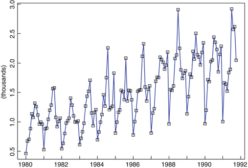
Figure shows the monthly sales (in kiloliters) of red wine by Australian winemakers from January 1980 through October 1991. In this case the set T 0 consists of the 142 times {(Jan. 1980), (Feb. 1980), ,(Oct. 1991)}. Given a set of n observations made at uniformly spaced time intervals, it is often convenient to rescale the time axis in such a way that T 0 becomes the set of integers {1,2,, n }. In the present example this amounts to measuring time in months with (Jan. 1980) as month 1. Then T 0 is the set {1,2,,142}. It appears from the graph that the sales have an upward trend and a seasonal pattern with a peak in July and a trough in January. To plot the data using ITSM, run the program by double-clicking on the ITSM icon and then select the option File>Project>Open>Univariate , click OK, and select the file WINE.TSM. The graph of the data will then appear on your screen.
Fig. 1.1
The Australian red wine sales, Jan. 1980Oct. 1991
Example 1.1.2
All-Star Baseball Games, 19331995
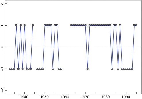
Figure shows the results of the all-star games by plotting x t , where
This is a series with only two possible values, 1. It also has some missing values, since no game was played in 1945, and two games were scheduled for each of the years 19591962.
Fig. 1.2
Results of the all-star baseball games, 19331995
Example 1.1.3
Accidental Deaths, U.S.A., 19731978; DEATHS.TSM
Like the red wine sales, the monthly accidental death figures show a strong seasonal pattern, with the maximum for each year occurring in July and the minimum for each year occurring in February. The presence of a trend in Figure we shall consider the problem of representing the data as the sum of a trend, a seasonal component, and a residual term.
Fig. 1.3
The monthly accidental deaths data, 19731978
Example 1.1.4
A Signal Detection Problem; SIGNAL.TSM
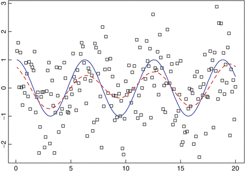
Figure shows simulated values of the series
where { N t } is a sequence of independent normal random variables, with mean 0 and variance 0.25. Such a series is often referred to as signal plus noise , the signal being the smooth function,

in this case. Given only the data X t , how can we determine the unknown signal component? There are many approaches to this general problem under varying assumptions about the signal and the noise. One simple approach is to smooth the data by expressing X t as a sum of sine waves of various frequencies (see Section . The waveform of the signal is quite close to that of the true signal in this case, although its amplitude is somewhat smaller.
Fig. 1.4
The series { X t } of Example
Example 1.1.5
Population of the U.S.A., 17901990; USPOP.TSM
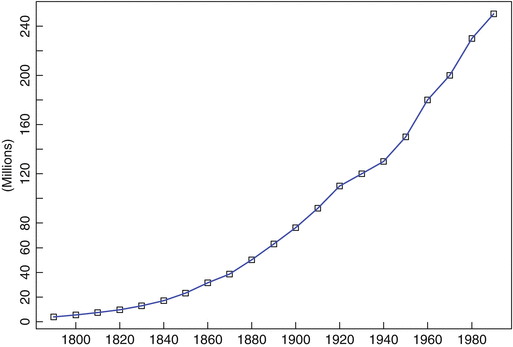
The population of the U.S.A., measured at 10-year intervals, is shown in Figure .
Fig. 1.5
Population of the U.S.A. at 10-year intervals, 17901990
Example 1.1.6
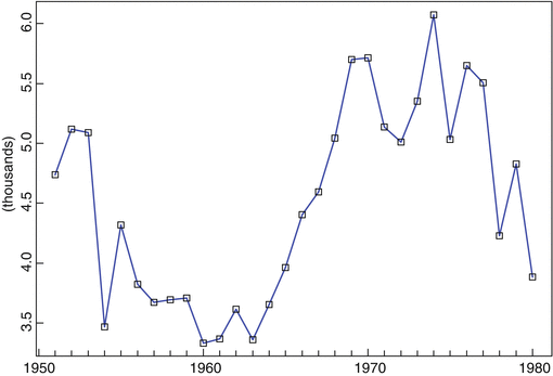
Number of Strikes Per Year in the U.S.A., 19511980; STRIKES.TSM
The annual numbers of strikes in the U.S.A. for the years 19511980 are shown in Figure . They appear to fluctuate erratically about a slowly changing level.
Fig. 1.6
Strikes in the U.S.A., 19511980
1.2 Objectives of Time Series Analysis
The examples considered in Section are an extremely small sample from the multitude of time series encountered in the fields of engineering, science, sociology, and economics. Our purpose in this book is to study techniques for drawing inferences from such series. Before we can do this, however, it is necessary to set up a hypothetical probability model to represent the data. After an appropriate family of models has been chosen, it is then possible to estimate parameters, check for goodness of fit to the data, and possibly to use the fitted model to enhance our understanding of the mechanism generating the series. Once a satisfactory model has been developed, it may be used in a variety of ways depending on the particular field of application.
The model may be used simply to provide a compact description of the data. We may, for example, be able to represent the accidental deaths data of Example , testing hypotheses such as global warming using recorded temperature data, predicting one series from observations of another, e.g., predicting future sales using advertising expenditure data, and controlling future values of a series by adjusting parameters. Time series models are also useful in simulation studies. For example, the performance of a reservoir depends heavily on the random daily inputs of water to the system. If these are modeled as a time series, then we can use the fitted model to simulate a large number of independent sequences of daily inputs. Knowing the size and mode of operation of the reservoir, we can determine the fraction of the simulated input sequences that cause the reservoir to run out of water in a given time period. This fraction will then be an estimate of the probability of emptiness of the reservoir at some time in the given period.



 in this case. Given only the data X t , how can we determine the unknown signal component? There are many approaches to this general problem under varying assumptions about the signal and the noise. One simple approach is to smooth the data by expressing X t as a sum of sine waves of various frequencies (see Section . The waveform of the signal is quite close to that of the true signal in this case, although its amplitude is somewhat smaller.







![Galit Shmueli - Practical Time Series Forecasting: A Hands-On Guide [2nd Edition]](/uploads/posts/book/82184/thumbs/galit-shmueli-practical-time-series-forecasting.jpg)