Bonaccorso - Hands-on unsupervised learning with Python : implement machine learning and deep learning models using Scikit-Learn, TensorFlow, and more

Another common method is called average linkage (or Unweighted Pair Group Method with Arithmetic Mean (UPGMA)). It is defined as follows:

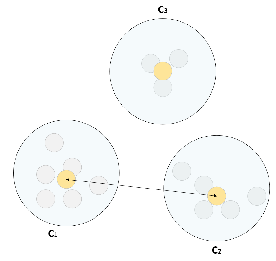
The idea is quite similar to complete linkage, but, in this case, the average of each cluster is taken into account and the goal is to minimize the average inter-cluster distance, considering all possible pairs (Ca, Cb). The following diagram shows an example of average linkage:

Average linkage is particularly helpful in bioinformatics applications (which is the main context in which hierarchical clustering has been defined). The mathematical explanation of its properties is non-trivial and I encourage you to check out the original paper (A Statistical Method for Evaluating Systematic Relationships, Sokal R., Michener C., University of Kansas Science Bulletin, 38, 1958) for further details.

In this chapter, we are going to introduce fundamental machine learning concepts, assuming that you have some basic knowledge of statistical learning and probability theory . You'll learn about the uses of machine learning techniques and t he logical process that improves our knowledge about both nature and the properties of a dataset . The purpose of the entire process is to build descriptive and predictive models the can support business decisions.

Unsupervised learning aims to provide tools for data exploration, mining, and generation. In this book, you'll explore different scenarios with concrete examples and analyses, and you'll learn how to apply fundamental and more complex algorithms to solve specific problems.

In this introductory chapter, we are going to discuss:

• Why do we need machine learning?
• Descriptive, diagnostic, predictive, and prescriptive analyses
• Types of machine learning
• Why are we using Python?

Data is everywhere. At this very moment, thousands of systems are collecting records that make up the history of specific services, together with logs, user interactions, and many other context-dependent elements. Only a decade ago, most companies couldn't even manage 1% of their data efficiently. For this reason, databases were periodically pruned and only important data used to be retained in permanent storage servers.

Conversely, nowadays almost every company can exploit cloud infrastructures that scale in order to cope with the increasing volume of incoming data. Tools such as Apache Hadoop or Apache Spark allow both data scientists and engineers to implement complex pipelines involving extremely large volumes of data. At this point, all the barriers have been torn down and a democratized process is in place. However, what is the actual value of these large datasets? From a business viewpoint, the information is valuable only when it can help make the right decisions, reducing uncertainty and providing better contextual insight. This means that, without the right tools and knowledge, a bunch of data is only a cost to the company that needs to be limited to increase the margins.

Machine learning is a large branch of computer science (in particular, artificial intelligence), which aims to implement descriptive and predictive models of reality by exploiting existing datasets. As this book is dedicated to practical unsupervised solutions, we are going to focus only on algorithms that describe the context by looking for hidden causes and relationships. However, even if only from a theoretical viewpoint, it's helpful to show the main differences between machine learning problems. Only complete awareness (not limited to mere technical aspects) of the goals can lead to a rational answer to the initial question, Why do we need machine learning?

We can start by saying that human beings have extraordinary cognitive abilities, which have inspired many systems, but they lack analytical skills when the number of elements increases significantly. For example, if you're a teacher who is meeting his/her class for the first time, you'll be able to compute a rough estimate of the percentage of female students after taking a glance at the entire group. Usually, the estimate is likely to be accurate and close to the actual count, even if the estimation is made by two or more individuals. However, if we repeat the experiment with the entire population of a school gathered in a courtyard, the distinction of gender will not be evident. This is because all students are clearly visible in the class; however, telling the sexes apart in the courtyard is limited by certain factors (for example, taller people can hide shorter ones). Getting rid of the analogy, we can say that a large amount of data usually carries a lot of information. In order to extract and categorize the information, it's necessary to take an automated approach.

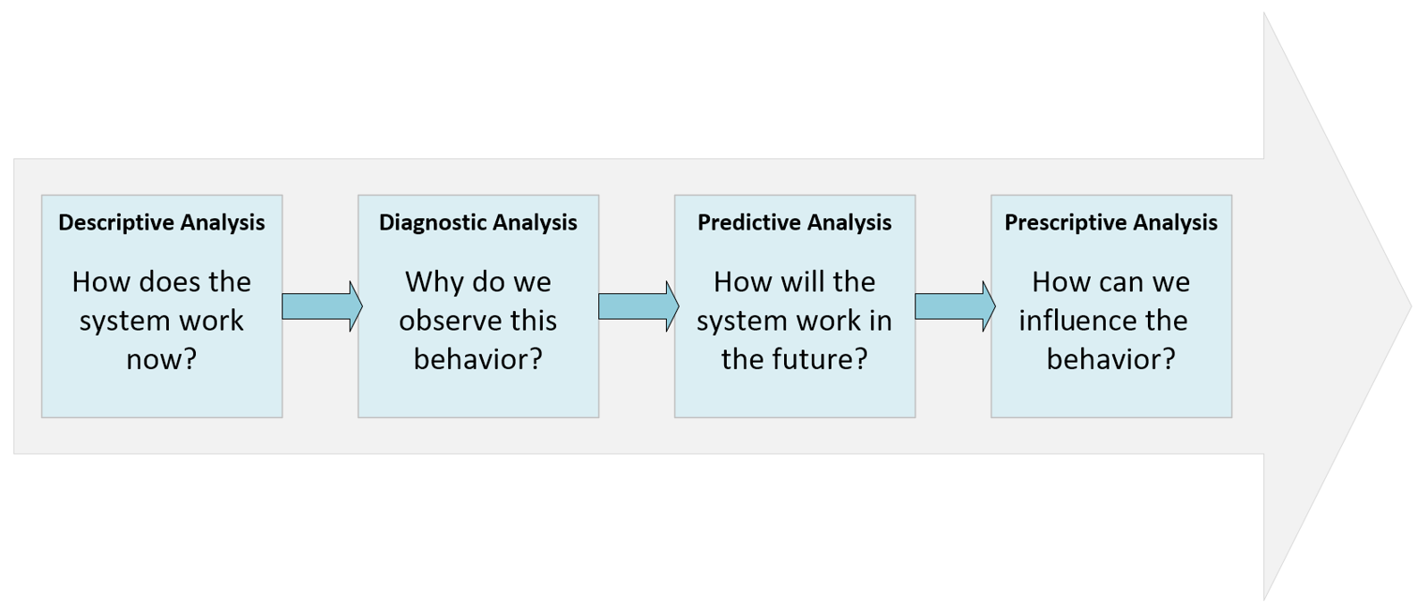
Before moving to the next section, let's discuss the concepts of descriptive, diagnostic, predictive, and prescriptive analyses, originally defined by Gartner. However, in this case, we want to focus on a system (for example, a generic context) that we are analyzing in order to gain more and more control over its behavior.

The complete process is represented in the following diagram:

This measure (together with all the other ones discussed from now on) is based on knowledge of the ground truth. Before introducing the index, it's helpful to define some common values. If we denote with Ytrue the set containing the true assignments and with Ypred, the set of predictions (both containing M values and K clusters), we can estimate the following probabilities:

In the previous formulas, ntrue/pred(k) represents the number of true/predicted samples belonging the cluster k K. At this point, we can compute the entropies of Ytrue and Ypred:

Considering the definition of entropy, H() is maximized by a uniform distribution, which, in its turn, corresponds to the maximum uncertainty of every assignment. For our purposes, it's also necessary to introduce the conditional entropies (representing the uncertainty of a distribution given the knowledge of another one) of Ytrue given Ypred and the other way around:

The function n(i, j) represents, in the first case, the number of samples with true label