Holmes - Introduction to Scientific Computing and Data Analysis

Introduction to Scientific Computing and Data Analysis — read online for free the complete book (whole text) full work

Below is the text of the book, divided by pages. System saving the place of the last page read, allows you to conveniently read the book "Introduction to Scientific Computing and Data Analysis" online for free, without having to search again every time where you left off. Put a bookmark, and you can go to the page where you finished reading at any time.

Light

Font size:

↓

↑

Georgia Tahoma Arial Verdana

Reset

Interval:

↓

↑

Bookmark:

Make

1234567...164

Springer International Publishing Switzerland 2016

Mark H. Holmes Introduction to Scientific Computing and Data Analysis Texts in Computational Science and Engineering 10.1007/978-3-319-30256-0_1

1. Introduction to Scientific Computing

Mark H. Holmes 1

(1)

Department of Mathematical Sciences, Rensselaer Polytechnic Institute, Troy, NY, USA

This chapter provides a brief introduction to the floating-point number system used in most scientific and engineering applications. A few examples are given in the next section illustrating some of the challenges using finite precision arithmetic, but it is worth quoting Donald Knuth to get things started. If you are unfamiliar with him, he was instrumental in the development of the analysis of algorithms, and is the creator of TeX. Anyway, here are the relevant quotes (Knuth []:

We dont know how much of the computers answers to believe. Novice computer users solve this problem by implicitly trusting in the computer as an infallible authority; they tend to believe that all digits of a printed answer are significant. Disillusioned computer users have just the opposite approach; they are constantly afraid that their answers are almost meaningless.

every well-rounded programmer ought to have a knowledge of what goes on during the elementary steps of floating point arithmetic. This subject is not at all as trivial as most people think, and it involves a surprising amount of interesting information.

One of the objectives in what follows is to help you from becoming disillusioned by identifying where problems can occur, and also to provide an appreciation for the difficulty of floating-point computation.

1.1 Unexpected Results

What follows are examples where the computed results are not what is expected. The reason for the problem is the same for each example. Namely, the finite precision arithmetic use by the computer generates errors that are significant enough that they affect the final result. Note that the calculations to follow are from MATLAB, but the same, or similar, results are expected for any system using double precision arithmetic (this is defined in Section ).

Example 1

Consider adding a series from largest to smallest

(1.1)

and the same series added from smallest to largest

(1.2)

According to the usual rules of arithmetic these are equal. However, this does not necessarily happen when the sums are calculated with a computer. If one calculates s ( n ) and S ( n ), and then calculates the difference S ( n ) s ( n ), the values given in Table are obtained. It is evident that for larger values of n , the two sums differ. The first question is why this happens, but there are other questions as well. For example, assuming both are incorrect, is it possible to determine which sum is closer to the exact result?

Table 1.1

Difference in partial sums for the harmonic series considered in Example .. Note that 8.9e

n	S ( n ) s ( n )
	8.88e 16
1,000	2.66e 15
10,000	3.73e 14
100,000	7.28e 14
1,000,000	7.83e 13

Example 2

Consider the function

(1.3)

If one expands this, the following is obtained

(1.4)

The expressions in () is not.

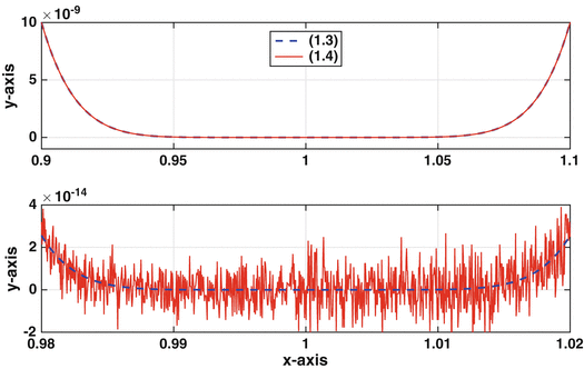
Figure 1.1

Plots of (). Upper graph: the interval is 0.9 x 1.1, and the two functions are so close that the curves are indistinguishable. Lower graph: the interval is 0.98 x 1.02, and now they are not so close.

Example 3

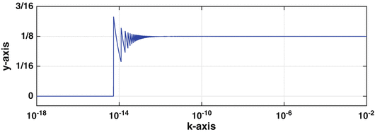
As a third example, consider the function

(1.5)

This is plotted in Figure . According to lHospitals rule

The computer agrees with this result for k down to about 1012 but for smaller values of k there is a problem. First, the function starts to oscillate and then, after k drops a little below 1014, the computer decides that y =0. It is also worth pointing out that ratios as in () comes from an approximation used to evaluate f (0), where .

Figure 1.2

Plot of ().

Example 4

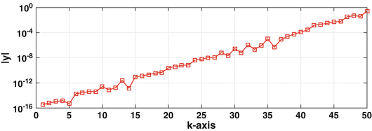
The final example concerns evaluating trigonometric functions, specifically, . It is well-known that if n is an integer, then . The integers of interest here are of the form , where k is a positive integer. Using MATLAB one finds that if k =52 then , while if k =53, then . Obviously, neither value is close to zero. To investigate this further, the absolute value of is plotted as a function of k in Figure . Interestingly, the error grows almost monotonically, eventually getting close to one. It is also worth pointing out that this result is not limited to MATLAB and as an example, the same curve is obtained if the valves are computed with Python.

Next page

1234567...164

Light

Font size:

↓

↑

Georgia Tahoma Arial Verdana

Reset

Interval:

↓

↑

Bookmark:

Make

Similar books «Introduction to Scientific Computing and Data Analysis»

Look at similar books to Introduction to Scientific Computing and Data Analysis. We have selected literature similar in name and meaning in the hope of providing readers with more options to find new, interesting, not yet read works.

Fabio Nelli

Pandas in 7 Days: Utilize Python to manipulate data, conduct scientific computing, time series analysis, and exploratory data analysis

Dhabaleswar K. Panda

High-Performance Big Data Computing (Scientific and Engineering Computation)

Dan Stanescu

A Gentle Introduction to Scientific Computing (Chapman & Hall/CRC Numerical Analysis and Scientific Computing Series)

McKinney

Python for Data Analysis: Data Wrangling with Pandas, NumPy, and IPython 2nd Edition

Wes McKinney

Python for Data Analysis

Dawn E. Holmes

Big Data: A Very Short Introduction

Robert Johansson

Numerical Python: Scientific Computing and Data Science Applications with Numpy, SciPy and Matplotlib

Mert Cuhadaroglu

Mastering Numerical Computing With NumPy: Master Scientific Computing and Perform Complex Operations With Ease

Wes McKinney

Python for Data Analysis: Data Wrangling with Pandas, NumPy, and IPython

Colina Coray

Introduction to scientific and technical computing

Cyrille Rossant

IPython Interactive Computing and Visualization Cookbook

Cyrille Rossant

Learning IPython for Interactive Computing and Data Visualization

Discussion, reviews of the book Introduction to Scientific Computing and Data Analysis and just readers' own opinions. Leave your comments, write what you think about the work, its meaning or the main characters. Specify what exactly you liked and what you didn't like, and why you think so.