Mert Cuhadaroglu - Mastering Numerical Computing With NumPy: Master Scientific Computing and Perform Complex Operations With Ease

As you will have noticed in the previous section, the distributions of our features are very dispersed. Handling the outliers in your model is a very important part of your analysis. It is also very crucial when you look at descriptive statistics. You can be easily confused and misinterpret the distribution because of these extreme values. SciPy has very extensive statistical functions for calculating your descriptive statistics in regards to trimming your data. The main idea of using the trimmed statistics is to remove the outliers (tails) in order to reduce their effect on statistical calculations. Let's see how we can use these functions and how they will affect our feature distribution:

To calculate the trimmed statistics, we used tmin(), tmax(), tvar(), and tmean(), as shown in the preceding code. All of these functions take limit values as a second parameter. In the CRIM feature, we can see many tails on the right side, so we limit the data to (1, 40) and then calculate the statistics. You can observe the difference by comparing the calculated statistics both before and after we have trimmed the values. As an alternative for tmean(), the trim_mean() function can be used if you want to slice your data proportionally from both sides. You can see how our mean and variance significantly changes after trimming the data. The variance is significantly decreased as we removed many extreme outliers between 40 and 89. The same trimming has a different effect on the mean, where the mean afterwards is more than doubled. The reason for this is that there were many zeros in the previous distribution, and by limiting the calculation between the values of 1 and 40, we removed all of these zeros, which resulted in a higher mean. Be advised that all of the preceding functions just trim your data on the fly while calculating these values, so the CRIM array is not trimmed. If you want to trim your data from both sides, you can use trimboth() and trim1() for one side. In both methods, instead of using limit values, you should use proportions as parameters. As an example, if you pass proportiontocut =0.2, it will slice your leftmost and rightmost values by 20%:

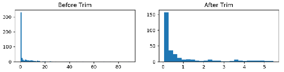
After trimming 20% of the values from both sides, we can interpret the distribution better and actually see that most of the values are between 0 and 1.5. It's hard to get this insight just by looking at the left histogram, as extreme values are dominating the histogram, and we can only see a single line around 0. As a result, trimmed functions are very useful in exploratory data analysis. In the next section, we will focus on box plots, which are very useful and popular graphical visuals for the descriptive analysis of data and outlier detection.

OpenBLAS

OpenBLAS is another optimized BLAS library, and it provides BLAS3-level optimizations for different configurations. Authors reported performance enhancements and improvements over BLAS that were comparable with Intel MKL's quality of performance.

Matrix decomposition

Matrix decomposition, or factorization methods, involves calculating the constituents of a matrix so that they can be used to simplify more demanding matrix operations. In practice, this means breaking the matrix you have into more than one matrix so that, when you calculate the product of these smaller matrices, you get your original matrix back. Some examples of matrix decomposition methods are singular-value decomposition (SVD), eigenvalue decomposition, Cholesky decomposition, lowerupper (LU), and QR decomposition.

Looking at basic statistics

In this section, you will start with the first step in statistical analysis by calculating the basic statistics of your dataset. Even though NumPy has limited built-in statistical functions, we can leverage its usage with SciPy. Before we start, let's describe how our analysis will flow. All of the feature columns and label columns are numerical, but you may have noticed that the Charles River dummy variable ( CHAS ) column has binary values (0,1), which means that it's actually encoded from categorical data. When you analyze your dataset, you can separate your columns into Categorical and Numerical. In order to analyze them all together, one type should be converted to another. If you have a categorical value and you want to convert it into a numeric value, you can do so by converting each category to a numerical value. This process is called encoding. On the other hand, you can perform binning by transforming your numerical values into category counterparts, which you create by splitting your data into intervals.

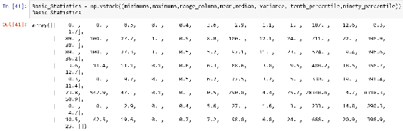
We will start our analysis by exploring its features one by one. In statistics, this method is known as univariate analysis. The purpose of univariate analysis mainly centered around description. We will calculate the minimum, maximum, range, percentiles, mean, and variance, and then we will plot some histograms and analyze the distribution of each feature. We will touch upon the concept of skewness and kurtosis and then look at the importance of trimming. After finishing our univariate analysis, we will continue with bivariate analysis, which means simultaneously analyzing two features. To do this, we will explore the relationship between two sets of features:

In [39]: np.set_printoptions(suppress=True, linewidth=125)
minimums = np.round(np.amin(samples, axis=0), decimals=1)
maximums = np.round(np.amax(samples, axis=0), decimals=1)
range_column = np.round(np.ptp(samples, axis=0), decimals=1)
mean = np.round(np.mean(samples, axis=0), decimals=1)
median = np.round(np.median(samples, axis=0), decimals=1)
variance = np.round(np.var(samples, axis=0), decimals=1)
tenth_percentile = np.round(np.percentile(samples, 10, axis=0), decimals = 1)
ninety_percentile = np.round(np.percentile(samples, 90 ,axis=0), decimals = 1)
In [40]: range_column
Out[40]: array([ 89. , 100. , 27.3, 1. , 0.5, 5.2, 97.1, 11. , 23. , 524. , 9.4, 396.6, 36.2])