Kattan - MATLAB for beginners: a gentle approach

This book is written for people who wish to learn MATLAB for the first time. The book is really designed for beginners and students. In addition, the book is suitable for students and researchers in various disciplines ranging from engineers and scientists to biologists and environmental scientists. The book is intended to be used as a first course in MATLAB in these areas. Students at both the undergraduate level and graduate level may benefit from this book. The material presented has been simplified to such a degree such that the book may also be used for students and teachers in high schools at least for performing simple arithmetic and algebraic manipulations. One of the objectives of writing this book is to introduce MATLAB and its powerful and simple computational abilities to students in high schools.

The material presented increases gradually in difficulty from the first few chapters on simple arithmetic operations to the last two chapters on solving equations and an introduction to calculus. In particular, the material presented in this book culminates in Chapters 6 and 7 on vectors and matrices, respectively. There is no discussion of strings, character variables or logical operators in this book. The emphasis is on computational and symbolic aspects. In addition, the MATLAB Symbolic Math Toolbox is emphasized in this book. A section is added at the end of each chapter (except chapters 1 and 9) dealing with various aspects of algebraic and symbolic computations with the Symbolic Math Toolbox. In fact, the final chapter on calculus assumes entirely the use of this toolbox.

Chapter 1 provides an overview of MATLAB and may be skipped upon a first reading of the book. The actual material in sequence starts in Chapter 2 which deals with arithmetic operations. Variables are introduced in Chapter 3 followed by mathematical functions in Chapter 4. The important topic of complex numbers is covered in Chapter 5. This is followed by Chapters 6 and 7 on vectors and matrices, respectively, which provide the main core of the book. In fact, MATLAB stands for MATrix LABoratory thus a long chapter is devoted to matrices and matrix computations. An introduction to programming using MATLAB is provided in Chapter 8. Plotting two-dimensional and three-dimensional graphs is covered in some detail in Chapter 9. Finally, the last two chapters (10 and 11) present solving equations and an introduction to calculus using MATLAB.

The material presented in this book has been tested with version 7 of MATLAB and should work with any prior or later versions. There are also over 230 exercises at the ends of chapters for students to practice. Detailed solutions to all the exercises are provided in the second half of the book. The material presented is very easy and simple to understand written in a gentle manner. An extensive references list is also provided at the end of the book with references to books and numerous web links for more information. This book will definitely get you started in MATLAB. The references provided will guide you to other resources where you can get more information.

I would like to thank my family members for their help and continued support without which this book would not have been possible. In this edition, I am providing two email addresses for my readers to contact me - .

August 2009

Peter I. Kattan

To suppress the output in MATLAB use a semicolon to end the command line as in the following examples. If the semicolon is not used then the output will be shown by MATLAB:

>> y = 30;
>> z = 8;
>> x = 2; y-z;
>> w = 4*y + 3*z
w =
144

MATLAB is case-sensitive, i.e. variables with lowercase letters are different than variables with uppercase letters. Consider the following examples using the variables x and X :

>> x = 1
x =
1
>> X = 2
X =
2
>> x
x =
1
>> X
X =
2

Use the help command to obtain help on any particular MATLAB command. The following example demonstrates the use of help to obtain help on the det command which calculated the determinant of a matrix:

>> help det
DET Determinant.
DET(X) is the determinant of the square matrix X.
Use COND instead of DET to test for matrix singularity.
See also cond.
Overloaded functions or methods (ones with the same name in other directories)
help sym/det.m
Reference page in Help browser doc det

The following examples show how to enter matrices and perform some simple matrix operations:

>> x = [1 2 3 ; 4 5 6 ; 7 8 9]
x =
123
456
789
>> y = [1 ; 0 ; -4]
y =
1
0
-4
>> w = x*y
w =
-11
-20
-29

Let us now see how to use MATLAB to solve a system of simultaneous algebraic equations. Let us solve the following system of simultaneous algebraic equations:

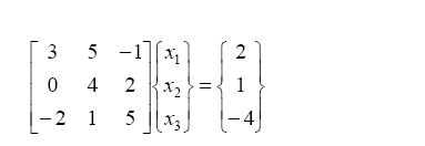
(1.1)

We will use Gaussian elimination to solve the above system of equations. This is performed in MATLAB by using the backslash operator \ as follows:

>> A= [3 5 -1 ; 0 4 2 ; -2 1 5]
A =
35 -1
042
-2 15
>> b = [2 ; 1 ; -4]
b =
2
1
-4
>> x = A\b
x =
-1.7692
1.1154
-1.7308

It is clear that the solution is x1 = -1.7692, x2 = 1.1154, and x3 = -1.7308. Alternatively, one can use the inverse matrix of A to obtain the same solution directly as follows:

>> x = inv(A)*b
x =
-1.7692
1.1154
-1.7308

It should be noted that using the inverse method usually takes longer than using Gaussian elimination especially for large systems of equations.