Richard A. Berk - Statistical Learning from a Regression Perspective

(1)

(2)

Richard A. Berk

Email:

As a first approximation, one can think of statistical learning as the muscle car version of Exploratory Data Analysis (EDA). Just as in EDA, the data can be approached with relatively little prior information and examined in a highly inductive manner. Knowledge discovery can be a key goal. But thanks to the enormous developments in computing power and computer algorithms over the past two decades, it is possible to extract information that would have previously been inaccessible. In addition, because statistical learning has evolved in a number of different disciplines, its goals and approaches are far more varied than conventional EDA.

In this book, the focus is on statistical learning procedures that can be understood within a regression framework. For a wide variety of applications, this will not pose a significant constraint and will greatly facilitate the exposition. The researchers in statistics, applied mathematics and computer science responsible for most statistical learning techniques often employ their own distinct jargon and have a penchant for attaching cute, but somewhat obscure, labels to their products: bagging, boosting, bundling, random forests, and others. There is also widespread use of acronyms: CART, LOESS, MARS, MART, LARS, LASSO, and many more. A regression framework provides a convenient and instructive structure in which these procedures can be more easily understood.

After a discussion of how statisticians think about regression analysis, this chapter introduces a number of key concepts and raises broader issues that reappear in later chapters. It may be a little difficult for some readers to follow parts of the discussion, or its motivation, the first time around. However, later chapters will flow far better with some of this preliminary material on the table, and readers are encouraged to return to the chapter as needed.

We begin by defining regression analysis. A common conception in many academic disciplines and policy applications equates regression analysis with some special case of the generalized Linear model: normal (linear) regression, binomial regression, Poisson regression, or other less common forms. Sometimes, there is more than one such equation, as in hierarchical models when the regression coefficients in one equation can be expressed as responses within other equations, or when a set of equations is linked though their response variables. For any of these formulations, inferences are often made beyond the data to some larger finite population or a data generation process. Commonly these inferences are combined with statistical tests, and confidence intervals. It is also popular to overlay causal interpretations meant to convey how the response distribution would change if one or more of the predictors were independently manipulated.

But statisticians and computer scientists typically start farther back. Regression is just about conditional distributions. The goal is to understand as far as possible with the available data how the conditional distribution of some response varies across subpopulations determined by the possible values of the predictor or predictors (Cook and Weisberg 1999: 27). That is, interest centers on the distribution of the response variable Y conditioning on one or more predictors X . Regression analysis fundamentally is the about conditional distributions: Y | X .

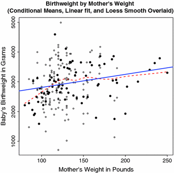
For example, Fig. Birthweight can be an important indicator of a newborns viability, and there is reason to believe that birthweight depends in part on the health of the mother. A mothers weight can be an indicator of her health.

In Fig. , the open circles are the observations. The filled circles are the conditional means and the likely summary statistics of interest. An inspection of the pattern of observations is by itself a legitimate regression analysis. Does the conditional distribution of birthweight vary depending on the mothers weight? If the conditional mean is chosen as the key summary statistic, one can consider whether the conditional means for infant birthweight vary with the mothers weight. This too is a legitimate regression analysis. In both cases, however, it is difficult to conclude much from inspection alone. The solid blue line is a linear least squares fit of the data. On the average, birthweight increases with the mothers weight, but the slope is modest (about 44 g for every 10 pounds), especially given the spread of the birthweight values. For many, this is a familiar kind of regression analysis. The dashed red line shows the fitted values for a smoother (i.e., lowess) that will be discussed in the next chapter. One can see that the linear relationship breaks down when the mother weighs less than about 100 pounds. There is then a much stronger relationship with the result that average birthweight can be under 2000 g (i.e., around 4 pounds). This regression analysis suggests that on the average, the relationship between birthweight and mothers weights is nonlinear.