• Complain

Eddelbuettel - Seamless R and C++ Integration with Rcpp

Here you can read online Eddelbuettel - Seamless R and C++ Integration with Rcpp full text of the book (entire story) in english for free. Download pdf and epub, get meaning, cover and reviews about this ebook. City: New York;Dordrecht, year: 2013, publisher: Springer, genre: Home and family. Description of the work, (preface) as well as reviews are available. Best literature library LitArk.com created for fans of good reading and offers a wide selection of genres:

Romance novel Science fiction Adventure Detective Science History Home and family Prose Art Politics Computer Non-fiction Religion Business Children Humor

Choose a favorite category and find really read worthwhile books. Enjoy immersion in the world of imagination, feel the emotions of the characters or learn something new for yourself, make an fascinating discovery.

Eddelbuettel Seamless R and C++ Integration with Rcpp
  • Book:
    Seamless R and C++ Integration with Rcpp
  • Author:
  • Publisher:
    Springer
  • Genre:
  • Year:
    2013
  • City:
    New York;Dordrecht
  • Rating:
    5 / 5
  • Favourites:
    Add to favourites
  • Your mark:
    • 100
    • 1
    • 2
    • 3
    • 4
    • 5

Seamless R and C++ Integration with Rcpp: summary, description and annotation

We offer to read an annotation, description, summary or preface (depends on what the author of the book "Seamless R and C++ Integration with Rcpp" wrote himself). If you haven't found the necessary information about the book — write in the comments, we will try to find it.

Preface; Target Audience; Historical Context; RelatedWork; Typographic Convention; Acknowledgements; Contents; List of Tables; List of Figures; List of Listings; Part I Introduction; 1 A Gentle Introduction to Rcpp; 1.1 Background: From R to C++; 1.2 A First Example; 1.2.1 Problem Setting; 1.2.2 A First R Solution; 1.2.3 A First C++ Solution; 1.2.4 Using Inline; 1.2.5 Using Rcpp Attributes; 1.2.6 A Second R Solution; 1.2.7 A Second C++ Solution; 1.2.8 A Third R Solution; 1.2.9 A Third C++ Solution; 1.3 A Second Example; 1.3.1 Problem Setting; 1.3.2 R Solution; 1.3.3 C++ Solution.

1.3.4 Comparison1.4 Summary; 2 Tools and Setup; 2.1 Overall Setup; 2.2 Compilers; 2.2.1 General Setup; 2.2.2 Platform-Specific Notes; 2.3 The R Application Programming Interface; 2.4 A First Compilation with Rcpp; 2.5 The Inline Package; 2.5.1 Overview; 2.5.2 Using Includes; 2.5.3 Using Plugins; 2.5.4 Creating Plugins; 2.6 Rcpp Attributes; 2.7 Exception Handling; Part II Core Data Types; 3 Data Structures: Part One; 3.1 The RObject Class; 3.2 The IntegerVector Class; 3.2.1 A First Example: Returning Perfect Numbers; 3.2.2 A Second Example: Using Inputs.

3.2.3 A Third Example: Using Wrong Inputs3.3 The NumericVector Class; 3.3.1 A First Example: Using Two Inputs; 3.3.2 A Second Example: Introducing clone; 3.3.3 A Third Example: Matrices; 3.4 Other Vector Classes; 3.4.1 LogicalVector; 3.4.2 CharacterVector; 3.4.3 RawVector; 4 Data Structures: Part Two; 4.1 The Named Class; 4.2 The List aka GenericVector Class; 4.2.1 List to Retrieve Parameters from R; 4.2.2 List to Return Parameters to R; 4.3 The DataFrame Class; 4.4 The Function Class; 4.4.1 A First Example: Using a Supplied Function; 4.4.2 A Second Example: Accessing an R Function.

4.5 The Environment Class4.6 The S4 Class; 4.7 ReferenceClasses; 4.8 The R Mathematics Library Functions; Part III Advanced Topics; 5 Using Rcpp in Your Package; 5.1 Introduction; 5.2 Using Rcpp.package.skeleton; 5.2.1 Overview; 5.2.2 R Code; 5.2.3 C++ Code; 5.2.4 DESCRIPTION; 5.2.5 Makevars and Makevars.win; 5.2.6 NAMESPACE; 5.2.7 Help Files; 5.2.7.1 mypackage-package. Rd; 5.2.7.2 rcpp_hello_world. Rd; 5.3 Case Study: The wordcloud Package; 5.4 Further Examples; 6 Extending Rcpp; 6.1 Introduction; 6.2 Extending Rcpp::wrap; 6.2.1 Intrusive Extension; 6.2.2 Nonintrusive Extension.

6.2.3 Templates and Partial Specialization6.3 Extending Rcpp::as; 6.3.1 Intrusive Extension; 6.3.2 Nonintrusive Extension; 6.3.3 Templates and Partial Specialization; 6.4 Case Study: The RcppBDT Package; 6.5 Further Examples; 7 Modules; 7.1 Motivation; 7.1.1 Exposing Functions Using Rcpp; 7.1.2 Exposing Classes Using Rcpp; 7.2 Rcpp Modules; 7.2.1 Exposing C++ Functions Using Rcpp Modules; 7.2.1.1 Documentation for Exposed Functions Using Rcpp Modules; 7.2.1.2 Formal Arguments Specification; 7.2.2 Exposing C++ Classes Using Rcpp Modules; 7.2.2.1 Initial Example.

7.2.2.2 Exposing Constructors Using Rcpp Modules.

Rcpp is the glue that binds the power and versatility of R with the speed and efficiency of C++. With Rcpp, the transfer of data between R and C++ is nearly seamless, and high-performance statistical computing is finally accessible to most R users. Rcpp should be part of every statisticians toolbox. -- Michael Braun, MIT Sloan School of Management Seamless R and C++ integration with Rcpp is simply a wonderful book. For anyone who uses C/C++ and R, it is an indispensable resource. The writing is outstanding. A huge bonus is the section on applications. This section covers the matrix pa.

Eddelbuettel: author's other books


Who wrote Seamless R and C++ Integration with Rcpp? Find out the surname, the name of the author of the book and a list of all author's works by series.

Seamless R and C++ Integration with Rcpp — read online for free the complete book (whole text) full work

Below is the text of the book, divided by pages. System saving the place of the last page read, allows you to conveniently read the book "Seamless R and C++ Integration with Rcpp" online for free, without having to search again every time where you left off. Put a bookmark, and you can go to the page where you finished reading at any time.

Light

Font size:

Reset

Interval:

Bookmark:

Make
Part 1
Introduction
Dirk Eddelbuettel Use R! Seamless R and C++ Integration with Rcpp 2013 10.1007/978-1-4614-6868-4_1 The Author 2013
1. A Gentle Introduction to Rcpp
Dirk Eddelbuettel 1
(1)
River Forest, Illinois, USA
Abstract
This initial chapter provides a first introduction to Rcpp . It uses a somewhat slower pace and generally more gentle approach than the rest of the book in order to show key concepts which are revisited and discussed in more depth throughout the remainder. So the aim of this chapter is to cover a fairly wide range of material, but at a more introductory level for an initial overview. Two larger examples are studied in detail. We first compute the Fibonacci sequence in three different ways in two languages. Second, we simulate from a multivariate dynamic model provided by a vector autoregression.
1.1 Background: From R to C++
R is both a powerful interactive environment for data analysis, visualization, and modeling and an expressive programming language designed and built to support these tasks. The interactive nature of working with datathrough data displays, summaries, model estimation, simulation, and numerous other tasksis a key strength of the R environment. And, so is the R programming language which permits use from interactive explorations to small scripts and all the way to complete implementations of new functionality. This R programming language is in fact a dialect of the S programming language initially developed by Bell Labs.
The dual nature of interactive analysis, as well as programming, is no accident. As succinctly expressed in the title of one of the books on the S language (which has provided the foundations upon which R is built), it is designed to support Programming with Data (Chambers ). That is a rather unique proposition as far as programming languages go. As a domain-specific language (DSL), R is tailored specifically to support and enable data analysis work. Moreover, there is also a particular focus on research use for developing new and exciting approaches, as well as solidifying existing approaches. R and its predecessor S are not static languages: they have evolved since the first designs well over thirty years ago and continue to evolve today.
To mention just one example of this evolution, object orientation in R is supported by the S3 and S4 class systems, as well as the newer Reference Classes. Of course, such flexibility of having alternate approaches can also be seen as a weakness. It may lead to yet more material which language beginners may find perplexing, and it may lead to small inconsistencies which may confuse intermediate and advanced users. Coincidentally, similar concerns are also sometimes raised about the C++ language. These arguments have some merit, but on the margin more useful and actually used languages are preferable to those that are very cleanly designed, yet not used much.
Having a proper programming language is a key feature supporting rigorous and reproducible research: by encoding all steps of a data analysis and estimation in a script or program, the analyst makes every aspect of the process explicit and thereby ensures full reproducibility.
Consider the first example which is presented below. It is a slightly altered version of an example going back to a post by Greg Snow to the r-help mailing list.
Listing 1.1 Plotting a density in R
1 xx <- faithful$eruptions
fit <- density(xx)
3 plot(fit)
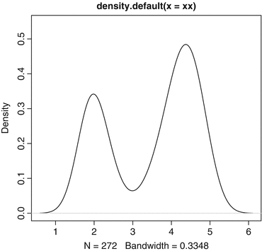
We assign a new variable xx by extracting the named component eruptions of the (two-column) data.frame faithful included with the R system. The data set contains waiting times between eruptions, as well as eruption duration times, at the Old Faithful geyser in the Yellowstone National Park in the USA. To estimate the density function of eruption duration based on this data, we then call the R function density (which uses default arguments besides the data we pass in). This function returns an object we named fit , and the plot function then visualizes it as shown in the corresponding Fig..
Fig 11 Plotting a density in R This is a nice example and it illustrates - photo 1
Fig. 1.1
Plotting a density in R
This is a nice example, and it illustrates some features of R such as the object-oriented nature in which we can simply plot an object returned from a modeling function. However, this example was introduced primarily to provide the basis for an extension also provided by Greg Snow and shown in the next listing.
Listing 1.2 Plotting a density and bootstrapped confidence interval in R
1 xx <- faithful$eruptions
fit1 <- density(xx)
3 fit2 <- replicate(10000, {
x <- sample(xx,replace=TRUE);
5 density(x, from=min(fit1$x), to=max(fit1$x))$y
})
7 fit3 <- apply(fit2, 1, quantile,c(0.025,0.975))
plot(fit1, ylim=range(fit3))
9 polygon(c(fit1$x,rev(fit1$x)),
c(fit3[1,], rev(fit3[2,])),
11 col=grey, border=F)
lines(fit1)
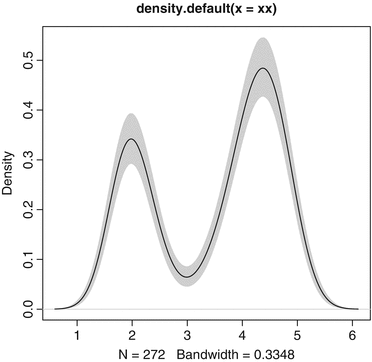
The first two lines are identical apart from now assigning to an object fit1 holding the estimated density. Lines three to six execute a minimal bootstrapping exercise. The replicate() function repeats N (here 10,000) times the code supplied in the second argument. Here, this argument is a code block delimited by braces, containing two instructions. The first instruction creates a new data set by resampling with replacement from the original data. The second instruction then estimates a density on this resampled data. This time the data range is limited to the range of the initial estimated in fit1 ; this ensures that the bootstrapped density is estimated on the same grid of x values as in fit1 . For this data set, the grid contains 512 points. We retain only the y coordinates of the fitthese will be collected as the N columns in the resulting object fit2 making this a matrix of dimension 512 N .
The next command on line 7 then applies the quantile() function to each of the 512 rows in fit2 , returning the 2.5 % and 97.5 % quantiles, and creating a new matrix of dimension 2 512 where the two rows contains the quantile estimates at each grid point for the x axis. We then plot the initial fit, adjusting the y -axis to the range of quantile estimates. Next, we add a gray polygon defined by the x grid and the quantile estimates which visualizes the bootstrapped 95 % confidence interval of the initial density estimate. Finally, we replot the fit1 density over the gray polygon. The resulting plot is shown in Fig..
Fig 12 Plotting a density and bootstrapped confidence interval in R The - photo 2
Fig. 1.2
Plotting a density and bootstrapped confidence interval in R
The main takeaway of this second example is that with just a handful of lines of code, we can deploy fairly sophisticated statistical modeling functions (such as the density estimate) and even provide a complete resampling strategy. This uses the same estimation function in a nonparametric bootstrap to also provide a confidence interval for the estimation, and finally plots both. Few languages besides R are this expressive and powerful for working with data.
A key aspect of the internal implementation of R is that its own core interpreter and extension mechanism are implemented in the C language. C is often used for system programming as it is reasonably lean and fast, yet also very portable and easily available on most hardware platforms. A key advantage of C is that it is extensible via external libraries and modules. R takes full advantage of this, and so does the Rcpp extension featured in this book. The principal goal of Rcpp is to make writing these extensions easier and less error-prone. The aim of this book is to show how this can be accomplished with what we consider relative ease compared to the standard C interface.
Next page
Light

Font size:

Reset

Interval:

Bookmark:

Make

Similar books «Seamless R and C++ Integration with Rcpp»

Look at similar books to Seamless R and C++ Integration with Rcpp. We have selected literature similar in name and meaning in the hope of providing readers with more options to find new, interesting, not yet read works.


Reviews about «Seamless R and C++ Integration with Rcpp»

Discussion, reviews of the book Seamless R and C++ Integration with Rcpp and just readers' own opinions. Leave your comments, write what you think about the work, its meaning or the main characters. Specify what exactly you liked and what you didn't like, and why you think so.