Carpenter James R. - Meta-Analysis with R

Meta-Analysis with R — read online for free the complete book (whole text) full work

Below is the text of the book, divided by pages. System saving the place of the last page read, allows you to conveniently read the book "Meta-Analysis with R" online for free, without having to search again every time where you left off. Put a bookmark, and you can go to the page where you finished reading at any time.

Light

Font size:

↓

↑

Georgia Tahoma Arial Verdana

Reset

Interval:

↓

↑

Bookmark:

Make

1234567...71

Part I
Getting Started

Springer International Publishing Switzerland 2015

Guido Schwarzer , James R. Carpenter and Gerta Rcker Meta-Analysis with R Use R! 10.1007/978-3-319-21416-0_1

1. An Introduction to Meta-Analysis in R

Guido Schwarzer 1, James R. Carpenter 2 and Gerta Rcker 1

(1)

Institute for Medical Biometry and Statistics, Medical Center University of Freiburg, Freiburg, Germany

(2)

MRC Clinical Trials Unit, London and London School of Hygiene and Tropical Medicine, London, UK

The world is awash with information. For any question, the briefest of internet searches will throw up a range of frequently contradictory answers. This underlies increasing awareness of the value of systematic evidence synthesisboth qualitative and quantitativeby researchers, policy makers and the broader public. It is reflected in the continuing development of the Cochrane Collaboration ( ].

Quantitative aspects have a key role to play in evidence synthesis. The statistical methodology for combining quantitative evidence from studies, known as meta-analysis, therefore features in almost every systematic review, and continues to undergo rapid development. A major concern of such developments is the need to detect and adjust for possible biases, as well as the synthesis of evidence from studies that have compared different combinations of interventions and measured these interventions with different outcomes.

The statistical software environment R [).

We believe that R is a natural choice for meta-analysis, as it provides the greatest range of methodology for meta-analysis in any single statistical software package. Our aim in writing this book is to introduce data analysts involved in meta-analysis, whether they are existing R users or not, to this software. No previous knowledge of R is assumed, and throughout the development is illustrated with worked examples. The data, and script files to repeat the examples, are downloadable from the website http://meta-analysis-with-r.org/ .

Established R users can probably skip the remainder of this chapter, in which we introduce some key R concepts and illustrate them with a simple meta-analysis. The aim in what follows is to get new users (who have used other statistics packages) started with R so that they can follow the presentation in the remainder of the book. For a more comprehensive introduction we recommend [].

The remainder of this chapter is best read alongside a computer running R. Thus, if you have not yet installed R, we would encourage you to do so: full installation details are given in Appendix A.1.

1.1 Getting Started with R

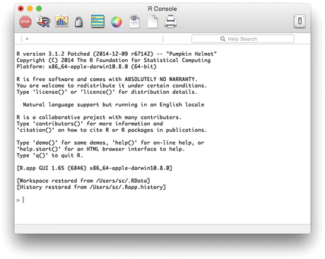
To start R either press on the R desktop icon created during installation or select the corresponding entry in the menu of installed applications. This should open the R Console window, an example of which in Mac OS X is shown in Fig.. R is not a menu driven program, so the user must either type commands at the command line, or execute a pre-written script. R is case sensitive, and most function names are in lower case. Typing the function name shows the code; to execute a function we must type parentheses. For example,

• type demo (followed by ), and R will print the code for the demo function,
• type demo() (followed by ), and R will open a window showing some of the demonstrations available.

Fig. 1.1

Screenshot of R Console window under Mac OS X

Towards the top of the list is the graphics demonstration. To run this, we need to give the argument graphics to the demo function, by placing it in the parentheses: demo(graphics) . Try this; you will need to press twice more to start the demonstration, and to move through the various plots. In summary: we pass information to R functions through the arguments which go between the parentheses that immediately follow function names.

1.1.1 Quitting R

To exit Rat the command line type q() . You will be asked Save workspace image? [y/n/c]: . Type one of y (yes: quit and save your data); n (no: quit without saving your data) or c (continue with R session), followed by . An alternative way to exit R is using the menu File Exit (under Windows) or R Quit (under Mac OS).

1.1.2 R as a Calculator

To begin, we note the following:

• Commands in R are typed into the R Console window to the right of the command prompt : >
• If R detects a command is not finished (for example, parentheses or quotes are not matched) then the next line will show the continuation prompt : +
  Either complete the command, or interrupt it by typing Ctrl+C under Linux.
• The # means that the remainder of the line will not be executed: we use this repeatedly to give a commentary on our R code.

Armed with this, we can start to explore R. In the R Console try the following commands (you do not need to type lines that begin with the # sign):

> # set x to be 2

> x <- 2

> # same assignment

> x = 2

> # display x

> x

[1] 2

> # set x to be the vector 1,2,3 using R function c

> x <- c(1,2,3)

> # same assignment

> x <- 1:3

> # display x

> x

[1] 1 2 3

> # add up the elements of x:

> sum(x)

[1] 6

> # set x to be a matrix

> x <- matrix(c(1,2,3,4), nrow=2)

> # display x

> x

[,1] [,2]

[1,] 1 3

[2,] 2 4

> # square the matrix x

> x*x

[,1] [,2]

[1,] 1 9

[2,] 4 16

> # square x and add 3 to all entries

> x*x + 3

[,1] [,2]

[1,] 4 12

[2,] 7 19

> # create a function, called f, which squares its argument

> f <- function(x){x*x}

> f(2)

[1] 4

> f(c(1,2,3))

[1] 1 4 9

> # square the matrix x using R function f

> f(x)

[,1] [,2]

[1,] 1 9

[2,] 4 16

1.1.3 Getting Help

The easiest way to get help on a function, for example the ls function is to type a ? followed by the function name at the R prompt: ?ls . Equivalently, we can type help(ls) . Either will open a window giving details of how to use the function. For more extensive help, the command help.start() opens a window or tab in your web browser with links to all the documentation.

1.2 Loading, Saving and Restoring Data

Data are stored in R in a slightly different way to many other packages: instead of having a single dataset available at a time, we have instead a workspace (also called global environment or environment) that may be thought of as a virtual library or virtual directory, which can contain many datasets, together with other R objects such as functions. This workspace is stored as a file, with default name .RData under Mac/Linux/Unix and _RData under Windows. Not only can we have separate .RData files for different projects, we can make the contents of as many as we like available to R. This can cause some confusion if they contain different objects of the same name!

For this book, we will only need one .RData file. This we store in the current Working directory . To find the current working directory type getwd() at the R command line.

Next page

1234567...71

Light

Font size:

↓

↑

Georgia Tahoma Arial Verdana

Reset

Interval:

↓

↑

Bookmark:

Make

Similar books «Meta-Analysis with R»

Look at similar books to Meta-Analysis with R. We have selected literature similar in name and meaning in the hope of providing readers with more options to find new, interesting, not yet read works.

D. James Kennedy

Led by the Carpenter: Finding Gods Purpose for Your Life

Meta Berger

A Milwaukee Womans Life on the Left: The Autobiography of Meta Berger

Edward Carpenter

Civilisation: Its Cause and Cure: And Other Essays

Steven Simske

Meta-Analytics: Consensus Approaches and System Patterns for Data Analysis

Evangelos Evangelou

Meta-Research: Methods and Protocols

Tom Carpenter

Woodworking

Thomas K Carpenter [Carpenter

Gladiators of Warsong

Sudharsan Ravichandiran

Hands-On Meta Learning with Python: Meta learning using one-shot learning, MAML, Reptile, and Meta-SGD with TensorFlow

John E. Hunter

Methods of Meta-Analysis: Correcting Error and Bias in Research Findings

Art Carpenter

Carpenter’s Complete Guide to the SAS Macro Language

Cooper

Research synthesis and meta-analysis: a step-by-step approach

Mike Allen

Interpersonal Communication Research: Advances Through Meta-analysis

Discussion, reviews of the book Meta-Analysis with R and just readers' own opinions. Leave your comments, write what you think about the work, its meaning or the main characters. Specify what exactly you liked and what you didn't like, and why you think so.