Foreman - Data smart: using data science to transform information into insight

This book relies on you having a working knowledge of spreadsheets, and I'm going to assume that you already understand the basics. If you've never used a formula before in your life, then you've got a slight uphill battle here. I'd recommend going through a For Dummies book or some other intro-level tutorial for Excel before diving into this.

That said, even if you're a seasoned Excel veteran, there's some functionality that'll keep cropping up in this text that you may not have had to use before. It's not difficult stuff; just things I've noticed not everyone has used in Excel. You'll be covering a wide variety of little features in this chapter, and the example at this stage might feel a bit disjointed. But you can learn what you can here, and then, when you encounter it organically later in the book, you can slip back to this chapter as a reference.

As Samuel L. Jackson says in Jurassic Park, Hold on to your butts!

Imagine you've been terribly unsuccessful in life, and now you're an adult, still living at home, running the concession stand during the basketball games played at your old high school. (I swear this is only semi-autobiographical.)

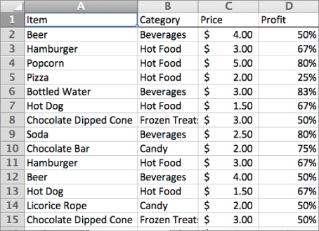
You have a spreadsheet full of last night's sales, and it looks like .

Concession stand sales

shows each sale, what the item was, what type of food or drink it was, the price, and the percentage of the sale going toward profit.

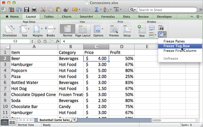
If you want to peruse the records, you can scroll down the sheet with your scroll wheel, track pad, or down arrow. As you scroll, it's helpful to keep the header row locked at the top of the sheet, so you can remember what each column means. To do that, choose Freeze Panes or Freeze Top Row from the View tab on Windows (Layout tab on Mac 2011 as shown in ).

Freezing the top row

To move quickly to the bottom of the sheet to look at how many transactions you have, you can select a value in one of the populated columns and press Ctrl+ (Command+ on a Mac). You'll zip right to the last populated cell in that column. In this sheet, the final row is 200. Also, note that using Ctrl/Command to jump around the sheet from left to right works much the same.

If you want to take an average of the sales prices for the night, below the price column, column C, you can jot the following formula:

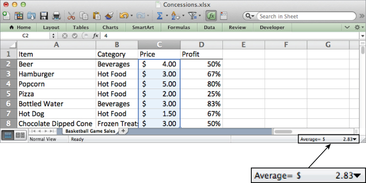
The average is $2.83, so you won't be retiring wealthy anytime soon. Alternatively, you can select the last cell in the column, C200, hold Shift+Ctrl+ to highlight the whole column, and then select the Average calculation from the status bar in the bottom right of the spreadsheet to see the simple summary statistic (see ). On Windows, you'll need to right-click the status bar to select the average if it's not there. On Mac, if your status bar is turned off, click the View menu and select Status Bar to turn it on.

Average of the price column in the status bar

Perhaps you'd like to view your profits in actual dollars rather than as percentages. You can add a header to column E called Actual Profit. In E2, you need only to multiply the price and profit columns together to obtain this:

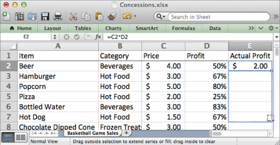
For beer, it's $2. You don't have to rewrite this formula in every cell in the column. Instead, Excel lets you grab the right-bottom corner of the cell and drag the formula where you like. The referenced cells in columns C and D will update relative to where you copy the formula. If, as in the case of the concession data, the column to the left is fully populated, you can double-click the bottom-right corner of the formula to have Excel fill the whole column (see ). Try this double-click action for yourself, because I'll be using it all over the place in this book, and if you get the hang of it now, you'll save yourself a whole lot of heartache.

Filling in a formula by dragging the corner

Now, what if you don't want the cells in the formula to change relative to the target when they're dragged or copied? Whatever you don't want changed, just add a $ in front of it.

For example, if you changed the formula in E2 to:

Then when you copy the formula down, nothing changes. The formula continues to reference row 2.

If you copy the formula to the right, however, C would become D, D would become E, and so on. If you don't want that behavior, you need to put a $ in front of the column references as well. This is called an absolute reference as opposed to a relative reference.

Excel offers static and dynamic options for formatting values. Take a look at column E, the Actual Profit column you just created. Select column E by clicking on the gray E column label. Then right-click the selection and choose Format Cells.

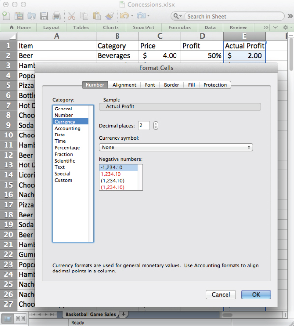
From within the Format Cells menu, you can tell Excel the type of number to be found in column E. In this case you want it to be Currency. And you can set the number of decimal places. Leave it at two decimals, as shown in . Also available in Format Cells are options for changing font colors, text alignment, fill colors, borders, and so on.

The Format Cells menu

But here's a conundrum. What if you want to format only the cells that have a certain value or range of values in them? And what if you want that formatting to change with the values?