Sarkar Dipayan. - Ensemble Machine Learning Cookbook

1. We first separate our feature and response set. We will also split our data into training and testing subsets in the following code block:

X = df_housingdata.iloc[:,1:14]
Y = df_housingdata.iloc[:,-1]
X_train, X_test, Y_train, Y_test = train_test_split(X, Y, random_state=1)

1. We will then create an instance of the DecisionTreeClassifier class and pass it to the BaggingClassifier() function:

dt_model = DecisionTreeRegressor()
bag_dt_model = BaggingRegressor(dt_model, max_features=1.0, n_estimators=5, bootstrap=True, random_state=1, )

1. We will fit our model to the training dataset as follows:

bag_dt_model.fit(X_train, Y_train)

1. We can see the model score in the following code block:

bag_dt_model.score(X_test, Y_test)

1. We use the predict() function and pass the test dataset to predict our target variable as follows:

predictedvalues = bag_dt_model.predict(X_test)

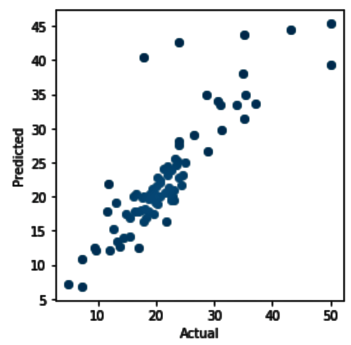
1. We plot the scatter plot of our actual values and the predicted values of our target variable with the following code:

#We can plot the actuals and the predicted values
plt.figure(figsize=(4, 4))
plt.scatter(Y_test, predictedvalues)
plt.xlabel('Actual')
plt.ylabel('Predicted')
plt.tight_layout()

Executing the preceding code gives us the following scatter plot:

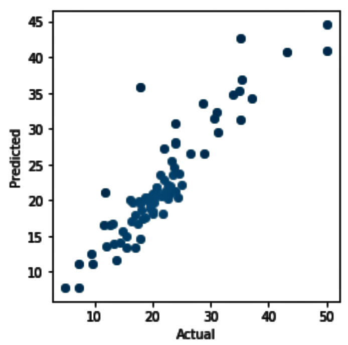
1. We now change the n_estimators parameter to 30 in the following code and re-execute the steps from Step 3 to Step 6:

bag_dt_model = BaggingRegressor(dt_model, max_features=1.0, n_estimators=30, bootstrap=True, random_state=1, )

This gives us the following score:

1. The plot of the actual values against the predicted values looks as follows. This shows us that the values are predicted more accurately than in our previous case when we changed the value of the n_estimator parameter from 5 to 30:

In Step 1, we looked at our dataset. In Step 2 and Step3, we looked at the statistics for the ham and spam class labels. In Step 4, we extended our analysis by looking at the word count and the character count for each of the messages in our dataset. In Step 5, we saw the distribution of our target variables (ham and spam), while in Step 6 we encoded our class labels for the target variable with the numbers 1 and 0. In Step 7, we split our dataset into training and testing samples. In Step 8, we used CountVectorizer() from sklearn.feature_extraction.text to convert the collection of messages to a matrix of token counts.

If you do not provide a dictionary in advance and do not use an analyzer that does some kind of feature selection, then the number of features will be equal to the vocabulary size found by analyzing the data. For more information on this, see the following: https://bit.ly/1pBh3T1.

In Step 9 and Step10, we built our model and imported the required classes from sklearn.metrics to measure the various scores respectively. In Step 11 and 12, we checked the accuracy of our training and testing datasets.

• The scikit-learn guide to sklearn.cross_validation.Bootstrap: https://bit.ly/2RC5MYv

In the following steps we will download the following packages:

To start with, import the os and pandas packages and set your working directory according to your requirements:

# import required packages
import os
import pandas as pd
# Set working directory as per your need
os.chdir(".../.../Chapter 2")
os.getcwd()

Download the Cryotherapy.csv dataset from GitHub and copy it to your working directory. Read the dataset:

df_cryotherapydata = pd.read_csv("Cryotherapy.csv")

Take a look at the data with the following code:

df_cryotherapydata.head(5)

We can see that the data has been read properly and has the Result_of_Treatment class variable. We then move on to creating models with Result_of_Treatment as the response variable.

In this section, we're going to use a dataset that contains information on default payments, demographics, credit data, payment history, and bill statements of credit card clients in Taiwan from April 2005 to September 2005. This dataset is taken from the UCI ML repository and is available at GitHub:

We will start by importing the required libraries:

# import os for operating system dependent functionalities
import os
# import other required libraries
import pandas as pd
from sklearn.preprocessing import StandardScaler
from sklearn.model_selection import train_test_split
from sklearn.linear_model import SGDClassifier
from sklearn.metrics import roc_curve
from sklearn.metrics import auc
import matplotlib.pyplot as plt

We set our working directory with the os.chdir() command:

# Set your working directory according to your requirement
os.chdir(".../Chapter 4/Logistic Regression")
os.getcwd()

Let's read our data. We will prefix the name of the DataFrame with df_ to make it easier to read:

df_creditdata = pd.read_csv("UCI_Credit_Card.csv")

We will now move on to look at building our model using SGDClassifier().

To start with, import the os and the pandas packages and set your working directory according to your requirements:

# import required packages
import os
import pandas as pd
import numpy as np
from sklearn.ensemble import AdaBoostClassifier
from sklearn.model_selection import GridSearchCV
from sklearn.model_selection import train_test_split
from sklearn.tree import DecisionTreeClassifier
from sklearn.metrics import roc_auc_score, roc_curve, auc
from sklearn.model_selection import train_test_split
# Set working directory as per your need
os.chdir(".../.../Chapter 8")
os.getcwd()

Download the breastcancer.csv dataset from GitHub and copy it to your working directory. Read the dataset:

df_breastcancer = pd.read_csv("breastcancer.csv")

Take a look at the first few rows with the head() function:

df_breastcancer.head(5)

Notice that the diagnosis variable has values such as M and B, representing Malign and Benign, respectively. We will perform label encoding on the diagnosis variable so that we can convert the M and B values into numeric values.

We use head() to see the changes:

# import LabelEncoder from sklearn.preprocessing
from sklearn.preprocessing import LabelEncoder
lb = LabelEncoder()
df_breastcancer['diagnosis'] =lb.fit_transform(df_breastcancer['diagnosis'])
df_breastcancer.head(5)

We then check whether the dataset has any null values:

df_breastcancer.isnull().sum()

We check the shape of the dataset with shape():

df_breastcancer.shape

We now separate our target and feature set. We also split our dataset into training and testing subsets:

# Create feature & response variables
# Drop the response var and id column as it'll not make any sense to the analysis
X = df_breastcancer.iloc[:,2:31]
# Target
Y = df_breastcancer.iloc[:,0]