Anurag Bhardwaj - Deep Learning Essentials

Torch is a Lua based deep learning framework developed by Ronan Collobert, Clement Farabet, and Koray Kavukcuoglu. It was initially used by the CILVR Lab at New York University . The Torch is powered by C/C++ libraries under its hood and also uses Compute Unified Device Architecture (CUDA) for its GPU interactions. It aims to be the fastest deep learning framework while also providing a simple C-like interface for rapid application development.

A distributed representation is dense, whereas each of the learned concepts is represented by multiple neurons simultaneously, and each neuron represents more than one concept. In other words, input data is represented on multiple, interdependent layers, each describing data at different levels of scale or abstraction. Therefore, the representation is distributed across various layers and multiple neurons. In this way, two types of information are captured by the network topology. On the one hand, for each neuron, it must represent something, so this becomes a local representation. On the other hand, so-called distribution means a map of the graph is built through the topology, and there exists a many-to-many relationship between these local representations. Such connections capture the interaction and mutual relationship when using local concepts and neurons to represent the whole. Such representation has the potential to capture exponentially more variations than local ones with the same number of free parameters. In other words, they can generalize non-locally to unseen regions. They hence offer the potential for better generalization because learning theory shows that the number of examples needed (to achieve the desired degree of generalization performance) to tune O (B) effective degrees of freedom is O (B). This is referred to as the power of distributed representation as compared to local representation (http://www.iro.umontreal.ca/~pift6266/H10/notes/mlintro.html).

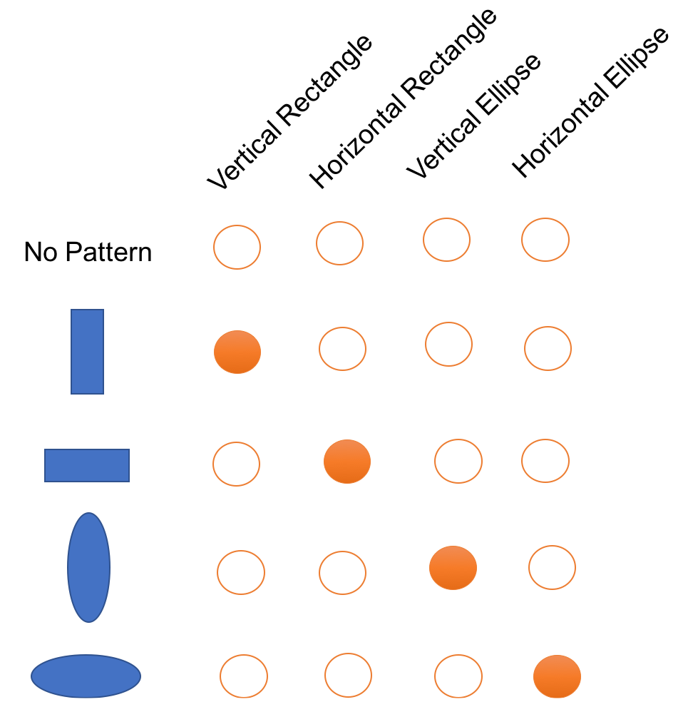
An easy way to understand the example is as follows. Suppose we need to represent three words, one can use the traditional one-hot encoding (length N), which is commonly used in NLP. Then at most, we can represent N words. The localist models are very inefficient whenever the data has componential structure:

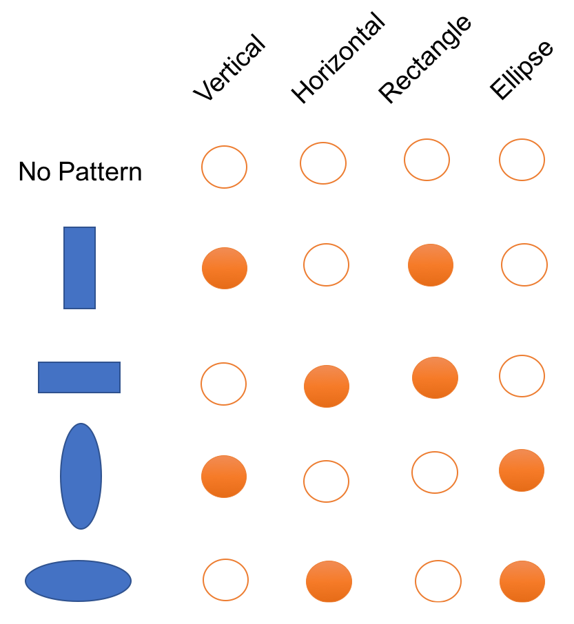
A distributed representation of a set of shapes would look like this:

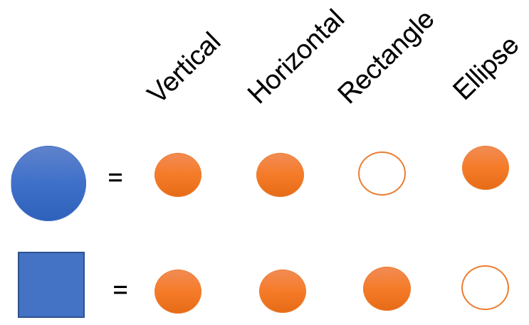
If we wanted to represent a new shape with a sparse representation, such as one-hot-encoding, we would have to increase the dimensionality. But whats nice about a distributed representation is we may be able to represent a new shape with the existing dimensionality. An example using the previous example is as follows:

Therefore, non-mutually exclusive features/attributes create a combinatorially large set of distinguishable configurations and the number of distinguishable regions grows almost exponentially with the number of parameters.

One more concept we need to clarify is the difference between distributed and distributional. Distributed is represented as continuous activation levels in a number of elements, for example, a dense word embedding, as opposed to one-hot encoding vectors.

On the other hand, distributional is represented by contexts of use. For example, Word2Vec is distributional, but so are count-based word vectors, as we use the contexts of the word to model the meaning.

One of the final layers in a CNN is often the fully connected layer, which is also known as a dense layer. Neurons in this layer are fully connected to all the activations in a previous layer. The output of this layer is usually the class score, where the number of neurons in this layer equals the number of classes typically.

Using the combination of the layers previously described, a CNN converts an input image to the final class scores. Each layer works in a different way and has different parameter requirements. The parameters in these layers are learned through a gradient descent-based algorithm in a back propagation way.

One of the important aspects of a CNN is that once it's trained, it learns a set of feature maps or filters, which act as feature extractors on natural scene images. As such, it would be great to visualize these filters and get an understanding of what the network has learned through its training. Fortunately, this is a growing area of interest with lots of tools and techniques that make it easier to visualize the trained filters by the CNN. There are two primary parts of the network that are interesting to visualize:

• Layer activation: This is the most common form of network visualization where one visualizes the activation of neurons during the forward pass of the network. This visualization is important for multiple reasons:
  • It allows you to see how each learned filter responds to each input image. You can use this information to get a qualitative understanding of what the filter has learned to respond to.
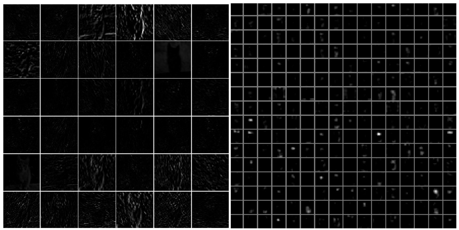
  • You can easily debug the network by seeing if most of the filters are learning any useful feature, or are simply blank images suggesting issues during network training. The following Visualizing activations of layers figure shows this step in more detail:

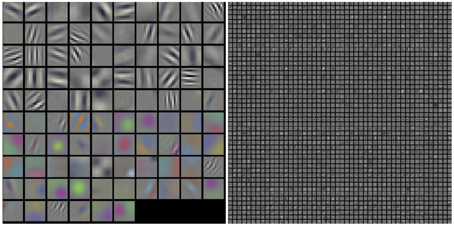
• Filter visualization: Another common use case for visualization is to visualize the actual filter values themselves. Remember that CNN filters can also be understood as feature detectors, which when visualized can demonstrate what kind of image feature each filter can extract. For example, the preceding Visualizing activations of layers figure illustrates that CNN filters can be trained to detect and extract edges in different orientations as well as different color combinations. Noisy filter values can also be easily detected during this technique to provide a feedback on poor training quality for the network:

In most cases, we should always consider ReLU first. But keep in mind that ReLU should only be applied to hidden layers. If your model suffers from dead neurons, then think about adjusting your learning rate, or try Leaky ReLU or maxout.