1. Modeling, Change, and Simulation
1.1 Feedback
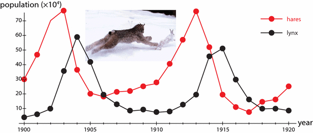
In the 1920s, ecologists began to study the populations of two Arctic species, lynx (a predator) and snowshoe hares (their prey) (Figure ). Notice that the populations oscillate . These oscillations are not random fluctuations; they have a roughly constant period of about 10 years. Note also that the rise and fall of the predator population systematically lags a little behind that of the prey population.
Figure 1.1:
Oscillations in the populations of lynx and snowshoe hares over time, from pelts of animals captured by
Hudson Bay Company trappers from 1900 to 1920.
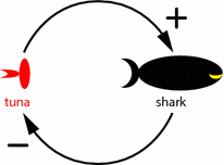
We want to understand what could be causing these oscillations. The first thing we have to realize is that finding the explanation requires us to take a careful look at the dynamic relationships between the two species. We have to make a model of their interactions. Even a very rough verbal model of the interaction reveals an interesting fact: the prey population positively affects the number of predators, while the predator population negatively affects the number of prey.
This makes the lynxhare system our first example of a system with negative feedback .
If we try to predict the systems behavior based on this verbal model, we discover a problem. Suppose we start with a certain number of predators and prey. What will happen? Well, the predators will eat some of the prey, and so the predator numbers will go up, and the prey numbers will go down, but then what? With high numbers of predators and low numbers of prey, the system cannot continue at the same pace; indeed, predator numbers will decline. But then what?
The problem here is that there is feedback in this system: the prey population affects the predator population and the predator population affects the prey population. It is difficult to predict the behavior of a feedback system based on this kind of verbal model. The diagram above has to be turned into a real mathematical model if we want to predict and understand the behavior.
The purpose of this book is to learn the art of making mathematical models of natural phenomena and learning how to predict behavior from them.
Interestingly, when we make a simple mathematical model of the predatorprey dynamics, it makes some nonobvious predictions.
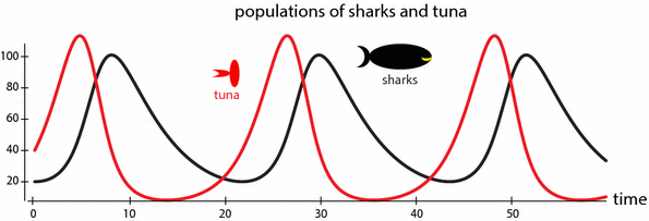
This first model will leave out weather fluctuations, disease outbreaks, plant abundance, the effects of crowding on behavior, and innumerable other things. It will include only birth, death, and predation. To underline the fact that this is a highly simplified model, we will call the predators sharks and the prey tuna . You will learn more about this model in Section . This kind of graph, which shows how quantities change over time, is called a time series .
Figure 1.2:
Behavior predicted by a model of interacting predator (shark) and prey (tuna) populations.
As you can see, the model predicts oscillations similar to the ones observed. What is the cause of these oscillations? The key to understanding this system is time delays . Sharks eat tuna, so the shark population grows and the tuna population diminishes until we get to a state where there are many sharks and very few tuna. The shark growth was caused by the previously high tuna levels, but now the tuna levels are low. The delayed shark growth has created a high-shark/low-tuna state, which means that the shark population will then decline, because due to the low tuna levels, very few sharks will be born and/or survive to maturity. This shark crash then takes the pressure off the tuna population, which then starts growing. The cycle then repeats.
Exercise 1.1.1
Copy two full cycles of the predatorprey oscillation time series in Figure and label the point at which each of the processes described in the above paragraph is occurring.
This introductory example features oscillations of two species, hares and lynx, but it has been noted that these data are actually not populations of animals, but rather populations of pelts , as collected by hunters. Therefore, some ecologists have argued that a better model for the populations would include two predators on the hares, lynx and hunters, each with their dynamics. This may well be true (Weinstein 1977). A model is a hypothesis about how to explain the data, and the merits of alternative models often must be considered.
Feedback Loops
The sharktuna system is an example of a system with feedback . The tuna population has a positive effect on the shark population, while the shark population has a negative effect on the tuna population (Figure ).
Figure 1.3:
Shark and tuna feedback dynamics.
More generally, in a feedback loop , the current state of a system affects the future state of that system by changing the inflows or outflows of the systems components. There are two types of feedback loops: positive and negative.
Positive Feedback
In positive feedback , a positive value of a variable leads to an increase in that variable, and a negative value of a variable leads to a decrease (more negative) in that variable.
For example, a person who has money will be able to invest it, bringing in more money. Or think of practicing a sport or musical instrument. Practice makes you better at the activity, which makes you enjoy it more, which makes you practice more. Positive feedback can also be bad, which might be casually referred to as negative. Think of a gambler who is losing badly, and so gambles more, ending up even further behind. In an arms race, one country can purchase more weapons, which causes its adversary to purchase more weapons, which causes the first country to purchase even more weapons. This is still positive feedback, just in a bad direction. Positive feedback reinforces change, so it can be thought of as reinforcing feedback.
There are many important examples of positive feedback loops:
Population growth Animals have young, which increases the population. The larger the population is, the more babies are born, which makes the population even larger. As long as resources are available, the population will keep growing.
CO

emissions Carbon dioxide emissions trap heat, which raises global temperatures. At higher temperatures, soil microbes have faster metabolic rates, which means that they break down soil organic matter faster, releasing even more CO


 emissions Carbon dioxide emissions trap heat, which raises global temperatures. At higher temperatures, soil microbes have faster metabolic rates, which means that they break down soil organic matter faster, releasing even more CO


