Cortez - Modern Optimization with R

Department of Information Systems, University of Minho, Guimares, Portugal

A vast number of real-world (often complex) tasks can be viewed as an optimization problem, where the goal is to minimize or maximize a given goal. In effect, optimization is quite useful in distinct application domains, such as Agriculture, Banking, Control, Engineering, Finance, Marketing, Production and Science. Moreover, due to advances in Information Technology, nowadays it is easy to store and process data. Since the 1970s, and following the Moores law, the number of transistors in computer processors has doubled every 2 years, resulting in more computational power at a reasonable price. And it is estimated that the amount of data storage doubles at a higher rate. Furthermore, organizations and individual users are currently pressured to increase efficiency and reduce costs. Rather than taking decisions based on human experience and intuition, there is an increasing trend for adopting computational tools, based on optimization methods, to analyze real-world data in order to make better informed decisions.

Optimization is a core topic of the Operations Research field, which developed several classical techniques, such as linear programming (proposed in the 1940s) and branch and bound (developed in the 1960s) (Schrijver ). In this book, we adopt the first term, modern optimization, to describe these algorithms.

In contrast with classical methods, modern optimization methods are general purpose solvers, i.e., applicable to a wide range of distinct problems, since few domain knowledge is required. For instance, the optimization problem does not need to be differentiable, which is required by classical methods such as gradient descent. There are only two main issues that need to be specified by the user when adopting modern heuristic methods (Michalewicz et al. ).

There is a vast number of successful real-world applications based on modern optimization methods. Examples studied by the author of this book include (among others): sitting guests at a wedding party (Rocha et al. ).

The R tool (R Core Team ) is an open source, high-level matrix programming language for statistical and data analysis. The tool runs on multiple platforms, including Windows , MacOS , Linux , FreeBSD , and other UNIX systems. R is an interpreted language, meaning that the user gets an immediate response of the tool, without the need of program compilation. The most common usage of R is under a console command interface, which often requires a higher learning curve from the user when compared with other more graphical user interface tools. However, after mastering the R environment, the user achieves a better understanding of what is being executed and higher control when compared with graphical interface based products.

The R base distribution includes a large variety of statistical techniques (e.g., distribution functions, statistical tests), which can be useful for inclusion in modern optimization methods and to analyze their results. Moreover, the tool is highly extensible by creating packages. The R community is very active and new packages are being continuously created, with more than 5,800 packages available at the Comprehensive R Archive Network (CRAN): for an example that optimizes data mining models).

To facilitate the usage of packages, given that a large number is available, several R packages are organized into CRAN task views. The Optimization and Mathematical Programming view is located at http://cran.r-project.org/web/views/Optimization.html and includes more than 60 packages. In this book, we explore several of these CRAN view packages (and others) related with modern optimization methods.

A major decision when using modern optimization methods is related with how to represent a possible solution (Michalewicz et al. ). Such decision sets the search space and its size, thus producing an impact on how new solutions are searched. To represent a solution, there are several possibilities. Binary, integer, character, real value and ordered vectors, matrices, trees and virtually any computer based representation form (e.g., computer program) can be used to encode solutions. A given representation might include a mix of different encodings (e.g., binary and real values). Also, a representation might be of fixed (e.g., fixed binary vectors) or of variable length (e.g., trees).

Historically, some of these representation types are attached with specific optimization methods. For instance, binary encodings are the basis of Genetic Algorithms (Holland ).

In what concerns this book, the representations adopted are restricted by the implementations available in the explored R tool packages, which mainly adopt binary or real values. Thus, there will be more focus on these type of representations. Nevertheless, Sect. ).

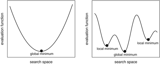
Another important decision for handling optimization tasks is the definition of the evaluation function, which should translate the desired goal (or goals) to be maximized or minimized. Such function allows to compare different solutions, by providing either a rank (ordinal evaluation function) or a quality measure score (numeric function) (Michalewicz et al. ). However, many practical problems are non-convex, often including noisy or complex function landscapes, with discontinuities. Optimization problems can even be dynamic, changing through time. For all these complex problems, an interesting alternative is to use modern optimization algorithms that only search a subset of the search space but tend to achieve near optimum solutions in a reasonable time.

By default, some implementations of optimization methods only perform a minimization of a numerical evaluation function. In such cases, a simple approach is to transform the maximization function max( f ( s )) into the equivalent minimization task min( f ( s )), by adopting , where s denotes the solution.

In several application fields (e.g., Control, Engineering, Finance) there are two or more goals that need to be optimized. Often, these goals conflict and trade-offs need to be set, since optimizing solutions under a single objective can lead to unacceptable outcomes in terms of the remaining goals. In such cases, a much better approach is to adopt a multi-objective optimization . In this book, we devote more attention to single response evaluation functions, since multi-objective optimization is discussed in a separated chapter (Chap.).

There are two main types of constraints (Michalewicz ): hard and soft . Hard constraints cannot be violated and are due to factors such as laws or physical restrictions. Soft constraints are related with other (often non-priority) user goals, such as increasing production efficiency while reducing environmental costs.

Soft restrictions can be handled by adopting a multi-objective approach (Chap. ): death-penalty, penalty-weights, repair and only generate feasible solutions.