Sandeep Nagar - Introduction to MATLAB for Engineers and Scientists: Solutions for Numerical Computation and Modeling

Introduction to MATLAB for Engineers and Scientists: Solutions for Numerical Computation and Modeling — read online for free the complete book (whole text) full work

Below is the text of the book, divided by pages. System saving the place of the last page read, allows you to conveniently read the book "Introduction to MATLAB for Engineers and Scientists: Solutions for Numerical Computation and Modeling" online for free, without having to search again every time where you left off. Put a bookmark, and you can go to the page where you finished reading at any time.

Light

Font size:

↓

↑

Georgia Tahoma Arial Verdana

Reset

Interval:

↓

↑

Bookmark:

Make

1234567...29

Sandeep Nagar 2017

Sandeep Nagar Introduction to MATLAB for Engineers and Scientists

1. Introduction to MATLAB

Sandeep Nagar 1

(1)

New York, USA

1.1 Introduction to Numerical Computing

With the advent of computers in the post World War II era, the need to simulate physical problems using this new tool led to the invention of numerical computing. Whereas analytical computation required pen, paper, and the human mind, numerical computation required a calculating device too. Successful implementation of computing devices to solve problems (especially involving repeated tasks) over a large array of data points was observed in many fields of science and engineering. For example, breaking enemys secret codes, simulating nuclear reactions before nuclear explosions, etc. The scope further expanded to civilian purposes , such as designing and simulating waterways, dams, electric power stations, town planning, etc. All of these applications need to use an equation or systems of equation for a physical model representing a physical problem. There are two ways that one can approach these equationsusing analytical and numerical techniques. We concentrate only on the numerical methods of solving equations using MATLAB in this book.

As time progressed, various schemes to define mathematical functions differentiation, integration, trigonometric, etc.were written for digital computers. This involved digitization, which certainly introduces errors. Knowledge of errors and their proper nullification could yield valuable information quicker than analytical results. Thus, it became one of the most actively researched fields of science and continues to be one. The search for faster and more accurate algorithms continues to drive innovation in the field of numerical computing and enables humanity to simulate otherwise impossible tasks.

1.2 Tools for Numerical Computing

As the numerical methods progressed as an alternative to analytical methods, computer programming languages were increasingly being used to codify them for programmed investigations of simulations. A number of options [] exist to perform numerical computation. Programming languages written to handle mathematical functions like FORTRAN, C, Python, Java, and Julia, to name a few, can be used to write algorithms for numerical computation.

1.2.1 The Need for Specialized Software

While all problems can be coded in programming languages, its necessary to change the approach to computing, file management, etc. when the microprocessor platform or operating system changes. This hinders interoperability. Modern programming languages address some of these issues, but the need for specialized software for numerical computingwhere predefined tools of numerical methods can be simply called as and when required and customized tools can be developedwas being felt in academia. A number of attempts were made in this direction.

1.2.2 The History of MATLAB

MATLAB was one such program and it was developed by Cleve Moler [], who was a math professor at the University of New Mexico, teaching numerical analysis and matrix theory. As a PhD student, he initially wrote a lot of code in FORTRAN to solve systems of simultaneous linear equations involving matrix algebra, which ultimately he called MATrixLABoratory (MATLAB). As a professor he wished his students could use the new packages without writing FORTRAN programs .

Hence, in late 1970s, the first version of MATLAB came out (written in FORTRAN). There were 80 functions for performing calculations involving linear algebra problems. Further down the line, Jack Little and Steve Bangert reprogrammed MATLAB in C with additional features for producing a commercial version of the software. Together, all three of them founded The MathWorks [].

Over a period of time, so many tools and features have been added to the base package of MATLAB that, along with this rich set of libraries, the installation requirements run it is many GBs of data. MATLAB became tremendously popular in the scientific community. It is used by more than 5,000 universities worldwide. It is sometimes rightly termed the language of engineering. Cheap availability of digital computing resources propelled its usage in industry and academia to such an extent that virtually every lab needs MATLAB now.

1.3 Installation Requirements

MATLAB should be purchased from the official web site of MathWorks [] installed with the base MATLAB package. This book discusses the usage of the base MATLAB package. Hence, to have a good experience with your MATLAB software, use a laptop or workstation with 1GB RAM and any of operating systems Windows, Linux, or MacOSX. Installation instructions are given with the product. The MATLAB environment is similar on all systems, so you need not worry about this while practicing with the book. This book has been tested for MATLAB R2017a version on the MacOSX 10.12 operating system.

1.4 Workspace

There are two ways to work within MATLAB. The first way is to work at the command line by writing one command at a time. The second method is to write a script (an .m file having a set of commands in a sequence) and run it from the command line by simply typing its name. For example, to run the a.m script file, you simply write the following at the command prompt:

1 >> a

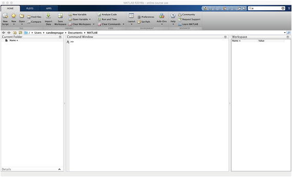
The command prompt is represented by the symbol >> by default. You enter a command at the command prompt and then press the Enter key to execute the command. See Figure .

Figure 1-1

MATLAB in action

1.4.1 The REPL Principle

The MATLAB command line works on the principle of REPL , which stands for Read-Evaluates-Prints-Loop. When input is fed into the MATLAB command prompt, the Julia language:

• Reads what the user types
• Evaluates what it reads
• Prints out the return value after evaluation
• Loops back and does it all over again

All MATLAB commands are treated as expressions to be evaluated at REPL. Many programming environments, such as Pythons interactive shell as well as the Jupyter notebook format, share the same approach. The new language called Julia also has a REPL and works in a similar fashion.

1.4.2 Calculator

In the simplest view, MATLAB works as a calculator with mathematical operators like multiplication ( * ), division ( / ), addition ( + ), subtraction ( - ), and exponentiation ( ^ ):

1 >> 3 + 5

2 ans = 8

3 >> 2 3

4 ans = 1

5 >> 3.0 * 5

6 ans = 15

7 >> 2 / 3

8 ans = 0.6667

9 >> format long

10 >> 2 / 3

11 ans = 0.666666666666667

12 >> format short

13 >> 2 / 3

14 ans = 0.6667

15 >> 2 % 3

16 ans = 2

17 >> 2 ^ 3

18 ans = 8

As seen in the previous example, when a command is fed into the command prompt >> , it is executed and an answer is given by displaying the results in the next line as ans = . To display more decimal digits in the result, you can use the format long command. By default, MATLAB works with the format short command.

1.4.3 Predefined Constants

1 >> pi

Next page

1234567...29

Light

Font size:

↓

↑

Georgia Tahoma Arial Verdana

Reset

Interval:

↓

↑

Bookmark:

Make

Similar books «Introduction to MATLAB for Engineers and Scientists: Solutions for Numerical Computation and Modeling»

Look at similar books to Introduction to MATLAB for Engineers and Scientists: Solutions for Numerical Computation and Modeling. We have selected literature similar in name and meaning in the hope of providing readers with more options to find new, interesting, not yet read works.

P K Thiruvikraman

Computational Methods Using MATLAB®: An introduction for physicists

Sulaymon L. Eshkabilov

Practical MATLAB Modeling: Programming Ordinary and Partial Differential Equations with Simulink

Nikolaos Ploskas

GPU Programming in MATLAB

Joseph Musto

Engineering Computation: An Introduction Using MATLAB and Excel

Ishchenko Anna

MATLAB Differential Equations

Sulaymon Eshkabilov

Beginning MATLAB and Simulink: From Novice to Professional

B. S. Grewal

Numerical Methods in Engineering and Science: C, C++, and MATLAB

Eihab B. M. Bashier

Practical Numerical and Scientific Computing with Matlab® and Python

Sandeep Nagar

Introduction to Python for Engineers and Scientists: Open Source Solutions for Numerical Computation

Sandeep Nagar

Introduction to Octave: For Engineers and Scientists

Sandeep Nagar

Introduction to Scilab: For Engineers and Scientists

César Pérez López

MATLAB Numerical Calculations

Discussion, reviews of the book Introduction to MATLAB for Engineers and Scientists: Solutions for Numerical Computation and Modeling and just readers' own opinions. Leave your comments, write what you think about the work, its meaning or the main characters. Specify what exactly you liked and what you didn't like, and why you think so.