Springer International Publishing Switzerland 2016
Klaus Neusser Time Series Econometrics Springer Texts in Business and Economics 10.1007/978-3-319-32862-1_1
1. Introduction and Basic Theoretical Concepts
Time series analysis is an integral part of every empirical investigation which aims at describing and modeling the evolution over time of a variable or a set of variables in a statistically coherent way. The economics of time series analysis is thus very much intermingled with macroeconomics and finance which are concerned with the construction of dynamic models. In principle, one can approach the subject from two complementary perspectives. The first one focuses on descriptive statistics . It characterizes the empirical properties and regularities using basic statistical concepts like mean, variance, and covariance. These properties can be directly measured and estimated from the data using standard statistical tools. Thus, they summarize the external (observable) or outside characteristics of the time series. The second perspective tries to capture the internal data generating mechanism . This mechanism is usually unknown in economics as the models developed in economic theory are mostly of a qualitative nature and are usually not specific enough to single out a particular mechanism. Thus, one has to consider some larger class of models. By far most widely used is the class of autoregressive moving-average (ARMA) models which rely on linear stochastic difference equations with constant coefficients. Of course, one wants to know how the two perspectives are related which leads to the important problem of identifying a model from the data.
The observed regularities summarized in the form of descriptive statistics or as a specific model are, of course, of principal interest to economics. They can be used to test particular theories or to uncover new features. One of the main assumptions underlying time series analysis is that the regularities observed in the sample period are not specific to that period, but can be extrapolated into the future. This leads to the issue of forecasting which is another major application of time series analysis.
Although its roots lie in the natural sciences and in engineering, time series analysis, since the early contributions by Frisch ( Each of these topics alone would justify the treatment of time series analysis in economics as a separate subfield.
1.1 Some Examples
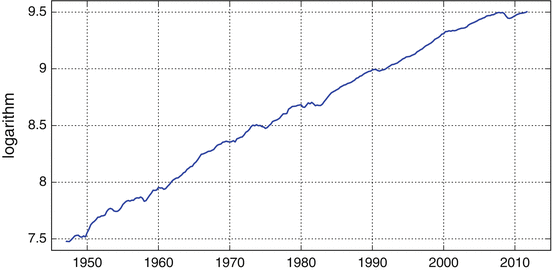
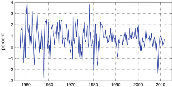
Before going into more formal analysis, it is useful to examine some prototypical economic time series by plotting them against time. This simple graphical inspection already reveals some of the issues encountered in this book. One of the most popular time series is the real gross domestic product. Figure which shows no trend anymore.
Fig. 1.1
Real gross domestic product (GDP) of the U.S. (chained 2005 dollars; seasonally adjusted annual rate)
Fig. 1.2
Quarterly growth rate of U.S. real gross domestic product (GDP) (chained 2005 dollars)
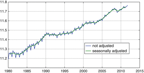
Another feature often encountered in economic time series is seasonality . This issue arises, for example in the case of real GDP, because of a particular regularity within a year: the first quarter being the quarter with the lowest values, the second and fourth quarter those with the highest values, and the third quarter being in between. These movements are due to climatical and holiday seasonal variations within the year and are viewed to be of minor economic importance. Moreover, these seasonal variations, because of there size, hide the more important business cycle movements. It is therefore customary to work with time series which have been adjusted for seasonality before hand. Figure shows the unadjusted and the adjusted real gross domestic product for Switzerland. The adjustment has been achieved by taking a moving-average. This makes the time series much smoother and evens out the seasonal movements.
Fig. 1.3
Comparison of unadjusted and seasonally adjusted Swiss real gross domestic product (GDP)
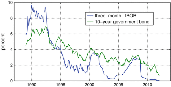
Other typical economic time series are interest rates plotted in Fig.. Over the period considered these two variables also seem to trend. However, the nature of this trend must be different because of the theoretically binding zero lower bound. Although the relative level of the two series changes over timeat the beginning of the sample, short-term rates are higher than long-terms onesthey move more or less together. This comovement is true in particular true with respect to the medium- and long-term.
Fig. 1.4
Short- and long-term Swiss interest rates (three-month LIBOR and 10 year government bond)
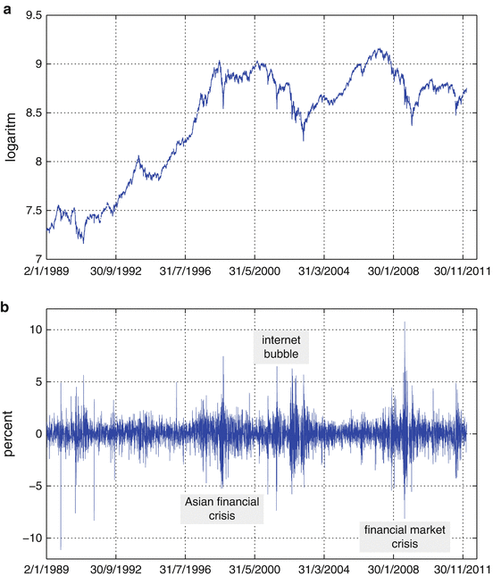
Other prominent time series are stock market indices. In Fig.
Fig. 1.5
Swiss Market Index (SMI). ( a ) Index. ( b ) Daily return
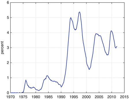
Finally, Fig.
Fig. 1.6
Unemployment rate in Switzerland
1.2 Formal Definitions
The previous section attempted to give an intuitive approach of the subject. The analysis to follow necessitates, however, more precise definitions and concepts. At the heart of the exposition stands the concept of a stochastic process. For this purpose we view the observation at some time t as the realization of random variable X t . In time series analysis we are, however, in general not interested in a particular point in time, but rather in a whole sequence. This leads to the following definition.
Definition 1.1.
A stochastic process {X t } is a family of random variables indexed by

and defined on some given probability space.
Thereby

denotes an ordered index set which is typically identified with time . In the literature one can encounter the following index sets:
Remark 1.1.
Given that

is identified with time and thus has a direction, a characteristic of time series analysis is the distinction between past, present, and future.






 and defined on some given probability space.
 denotes an ordered index set which is typically identified with time . In the literature one can encounter the following index sets:
 is identified with time and thus has a direction, a characteristic of time series analysis is the distinction between past, present, and future.