1.1 Introduction
A graph as a mathematical object may be defined as a pair

, where V is a set of vertices or nodes and E is a set of edges . Each edge is associated with a pair of nodes, its endpoints . Edges may in general be directed, undirected, or bidirected. Graphs are typically visualized by representing nodes by circles or points, and edges by lines, arrows, or bidirected arrows. We use the notation , , and to denote edges between and . Graphs are useful in a variety of applications, and a number of packages for working with graphs are available in R .
We have found the graph package to be particularly useful, since it provides a way of representing graphs as so-called graphNEL objects (graphs as N ode and E dge L ists) and thereby gives access to a wide range of graph-theoretic operations (in the graph package), efficient implementations of standard graph algorithms (in the RBGL package), and allows the graphs to be easily displayed in a variety of layouts (using the Rgraphviz package from BioConductor). Much of this book uses this representation. In statistical applications we are particularly interested in two special graph types: undirected graphs and directed acyclic graphs (often called DAGs).
We have also found the igraph package to be useful. Like the graph package, igraph supports both undirected and directed graphs and implements various graph algorithms. Functions in the package allow graphs to be displayed in a variety of formats. The internal representation of graphs in the igraph package differs from the representation in the graph package.
The gRbase package supplements graph and igraph by implementing some algorithms useful in graphical modelling. gRbase also provides two wrapper functions, ug() and dag() , for easily creating undirected graphs and DAGs represented either as graphNEL objects (the default), igraph objects or adjacency matrices.
The first sections of this chapter describe some of the most useful functions available when working with graphical models. These come variously from the gRbase , graph and RBGL packages, but it is not usually necessary to know which. To use the functions and plot the graphs it is enough to load gRbase and Rgraphviz , since gRbase automatically loads the other packages. To find out which package a function we mention belongs to, please refer to the index to this book or to the usual help functions.
As statistical objects, graphs are used to represent models, with nodes representing model variables (and sometimes model parameters) in such a way that the independence structure of the model can be read directly off the graph. Accordingly, a section of this chapter is devoted to a brief description of the key concept of conditional independence and explains how this is linked to graphs. Throughout the book we shall repeatedly return to this in more detail.
1.2 Graphs
Our graphs have a finite node set V and for the most part they are simple graphs in the sense that they have no loops nor multiple edges. Two vertices and are said to be adjacent , written , if there is an edge between and in

, i.e. if either , , or .
In this chapter we primarily represent graphs as graphNEL objects, and except where stated otherwise, the functions we describe operate on these objects. However, different representations can be useful for various reasons, for example igraph objects or as adjacency matrices. It is easy to convert between graphNEL objects, igraph objects and adjacency matrices, using the as() function. For example, if gNg is a graphNEL object, then
creates versions of the same graph represented as an igraph object and as an adjacency matrix. Similarly, to convert back we could write
1.2.1 Undirected Graphs
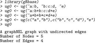
An undirected graph may be created using the ug() function. The graph can be specified using a list of formulas, a single formula or a list of vectors. Thus the following forms are equivalent:
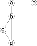
graphNEL graphs are displayed with plot() :
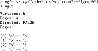
Per default the ug() function returns an graphNEL object, but the options result="igraph" or result="matrix" lead it to return an igraph or adjacency matrix instead. For example,
There is a plot() method for igraph objects in the igraph package. There are also various facilities for controlling the layout. For example, we may use a layout algorithm called layout.spring as follows:
The default size of vertices and their labels is quite small. This is easily changed by setting certain attributes on the graph, see Sect. for examples. However, to avoid changing these attributes for all the graphs shown in the following we have defined a small plot function myiplot() as follows:




 , where V is a set of vertices or nodes and E is a set of edges . Each edge is associated with a pair of nodes, its endpoints . Edges may in general be directed, undirected, or bidirected. Graphs are typically visualized by representing nodes by circles or points, and edges by lines, arrows, or bidirected arrows. We use the notation , , and to denote edges between and . Graphs are useful in a variety of applications, and a number of packages for working with graphs are available in R .
 , i.e. if either , , or .

