LitArk » Books » Home and family

Klette - Concise Computer Vision: an Introduction into Theory and Algorithms

Here you can read online Klette - Concise Computer Vision: an Introduction into Theory and Algorithms full text of the book (entire story) in english for free. Download pdf and epub, get meaning, cover and reviews about this ebook. City: London, year: 2014, publisher: Springer London, genre: Home and family. Description of the work, (preface) as well as reviews are available. Best literature library LitArk.com created for fans of good reading and offers a wide selection of genres:

Romance novel Science fiction Adventure Detective Science History Home and family Prose Art Politics Computer Non-fiction Religion Business Children Humor

Choose a favorite category and find really read worthwhile books. Enjoy immersion in the world of imagination, feel the emotions of the characters or learn something new for yourself, make an fascinating discovery.

Book:
Concise Computer Vision: an Introduction into Theory and Algorithms
Author:
Klette / Reinhard
Publisher:
Springer London
Genre:
Books / Home and family
Year:
2014
City:
London
Rating:
3 / 5
Favourites:
Add to favourites
Your mark:
- 60
- 1
- 2
- 3
- 4
- 5

Description
Author's other books
Similar books

Concise Computer Vision: an Introduction into Theory and Algorithms: summary, description and annotation

We offer to read an annotation, description, summary or preface (depends on what the author of the book "Concise Computer Vision: an Introduction into Theory and Algorithms" wrote himself). If you haven't found the necessary information about the book — write in the comments, we will try to find it.

Many textbooks on computer vision can be unwieldy and intimidating in their coverage of this extensive discipline. This textbook addresses the need for a concise overview of the fundamentals of this field. Concise Computer Vision provides an accessible general introduction to the essential topics in computer vision, highlighting the role of important algorithms and mathematical concepts. Classroom-tested programming exercises and review questions are also supplied at the end of each chapter. Topics and features: Provides an introduction to the basic notation and mathematical concepts for describing an image, and the key concepts for mapping an image into an image Explains the topologic and geometric basics for analysing image regions and distributions of image values, and discusses identifying patterns in an image Introduces optic flow for representing dense motion, and such topics in sparse motion analysis as keypoint detection and descriptor definition, and feature tracking using the Kalman filter Describes special approaches for image binarization and segmentation of still images or video frames Examines the three basic components of a computer vision system, namely camera geometry and photometry, coordinate systems, and camera calibration Reviews different techniques for vision-based 3D shape reconstruction, including the use of structured lighting, stereo vision, and shading-based shape understanding Includes a discussion of stereo matchers, and the phase-congruency model for image features Presents an introduction into classification and learning, with a detailed description of basic AdaBoost and the use of random forests This concise and easy to read textbook/reference is ideal for an introductory course at third- or fourth-year level in an undergraduate computer science or engineering programme.;Image Data -- Image Processing -- Image Analysis -- Dense Motion Analysis -- Image Segmentation -- Cameras, Coordinates and Calibration -- 3D Shape Reconstruction -- Stereo Matching -- Feature Detection and Tracking -- Object Detection.

Klette: author's other books

Who wrote Concise Computer Vision: an Introduction into Theory and Algorithms? Find out the surname, the name of the author of the book and a list of all author's works by series.

Concise Computer Vision: an Introduction into Theory and Algorithms — read online for free the complete book (whole text) full work

Below is the text of the book, divided by pages. System saving the place of the last page read, allows you to conveniently read the book "Concise Computer Vision: an Introduction into Theory and Algorithms" online for free, without having to search again every time where you left off. Put a bookmark, and you can go to the page where you finished reading at any time.

Light

Font size:

↓

↑

Reset

Interval:

↓

↑

Bookmark:

Make

Reinhard Klette Undergraduate Topics in Computer Science Concise Computer Vision 2014 An Introduction into Theory and Algorithms 10.1007/978-1-4471-6320-6_1

Springer-Verlag London 2014

1. Image Data

Reinhard Klette 1

(1)

Computer Science Department, University of Auckland, Auckland, New Zealand

Abstract

This chapter introduces basic notation and mathematical concepts for describing an image in a regular grid in the spatial domain or in the frequency domain. It also details ways for specifying colour and introduces colour images.

1.1 Images in the Spatial Domain

A (digital) image is defined by integrating and sampling continuous (analog) data in a spatial domain. It consists of a rectangular array of pixels ( x , y , u ), each combining a location Concise Computer Vision an Introduction into Theory and Algorithms - image 1

Concise Computer Vision an Introduction into Theory and Algorithms - image 1

and a value u , the sample at location ( x , y ). Concise Computer Vision an Introduction into Theory and Algorithms - image 2

is the set of all integers. Points Concise Computer Vision an Introduction into Theory and Algorithms - image 3

form a regular grid . In a more formal way, an image I is defined on a rectangular set, the carrier

11 of I containing the grid points or pixel locations for N cols 1 and N - photo 4

(1.1)

of I containing the grid points or pixel locations for N cols 1 and N rows 1.

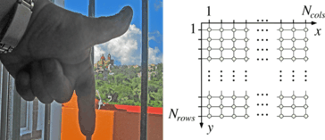
We assume a left-hand coordinate system as shown in Fig.. Row y contains grid points {(1, y ),(2, y ),,( N cols , y )} for 1 y N rows , and column x contains grid points {( x ,1),( x ,2),,( x , N rows )} for 1 x N cols .

Fig. 1.1

A left-hand coordinate system. The thumb defines the x -axis, and the pointer the y -axis while looking into the palm of the hand. (The image on the left also shows a view on the baroque church at Valenciana, always present outside windows while this book was written during a stay of the author at CIMAT Guanajuato)

This section introduces into the subject of digital imaging by discussing ways to represent and to describe image data in the spatial domain defined by the carrier .

1.1.1 Pixels and Windows

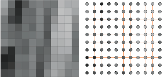
Figure illustrates two ways of thinking about geometric representations of pixels, which are samples in a regularly spaced grid.

Fig. 1.2

Left : When zooming into an image, we see shaded grid squares ; different shades represent values in a chosen set of image values. Right : Image values can also be assumed to be labels at grid points being the centres of grid squares

Grid Cells, Grid Points, and Adjacency

Images that we see on a screen are composed of homogeneously shaded square cells. Following this given representation, we may think about a pixel as a tiny shaded square. This is the grid cell model . Alternatively, we can also consider each pixel as a grid point labelled with the image value. This grid point model was already indicated in Fig..

Insert 1.1

(Origin of the Term Pixel)

The term pixel is short for picture element. It was introduced in the late 1960 s by a group at the Jet Propulsion Laboratory in Pasadena , California , that was processing images taken by space vehicles . See [R.B. Leighton, N.H. Horowitz, A.G. Herriman, A.T. Young, B.A. Smith, M.E. Davies, and C.B. Leovy. Mariner 6 television pictures: First report. Science , :684690, 1969].

Pixels are the atomic elements of an image. They do not define particular adjacency relations between pixels per se. In the grid cell model we may assume that pixel locations are adjacent iff they are different and their tiny shaded squares share an edge. Alternatively, we can also assume that they are adjacent iff they are different and their tiny shaded squares share at least one point (i.e. an edge or a corner).

Image Windows

A window

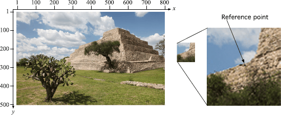
is a subimage of image I of size m n positioned with respect to a reference point p (i.e., a pixel location). The default is that m = n is an odd number, and p is the centre location in the window. Figure shows the window SanMiguel Fig 13 A 7377 window in the image SanMiguel The marked - photo 8

( SanMiguel ).

Fig. 1.3

A 7377 window in the image SanMiguel . The marked reference pixel location is at p =(453,134) in the image that shows the main pyramid at Caada de la Virgin, Mexico

Usually we can simplify the notation to W p because the image and the size of the window are known by the given context.

1.1.2 Image Values and Basic Statistics

Image values u are taken in a discrete set of possible values. It is also common in computer vision to consider the real interval

as the range of a scalar image. This is in particular of value if image values are interpolated within performed processes and the data type REAL is used for image values. In this book we use integer image values as a default.

Scalar and Binary Images

A scalar image has integer values u {0,1,,2 a 1}. It is common to identify such scalar values with grey levels, with 0=black and 2 a 1=white; all other grey levels are linearly interpolated between black and white. We speak about grey-level images in this case. For many years, it was common to use a =8; recently a =16 became the new technological standard. In order to be independent, we use G max=2 a 1.

A binary image has only two values at its pixels, traditionally denoted by 0=white and 1=black, meaning black objects on a white background.

Vector-Valued and RGB Images

A vector-valued image has more than one channel or band , as it is the case for scalar images. Image values Concise Computer Vision an Introduction into Theory and Algorithms - image 11

Concise Computer Vision an Introduction into Theory and Algorithms - image 11

are vectors of length N channels . For example, colour images in the common RGB colour model have three channels, one for the red component, one for the green, and one for the blue component. The values u i in each channel are in the set {0,1,, G max}; each channel is just a grey-level image. See Fig..

Fig 14 Original RGB colour image Fountain upper left showing a square in - photo 12

Light

Font size:

↓

↑

Reset

Interval:

↓

↑

Bookmark:

Make

Similar books «Concise Computer Vision: an Introduction into Theory and Algorithms»

Look at similar books to Concise Computer Vision: an Introduction into Theory and Algorithms. We have selected literature similar in name and meaning in the hope of providing readers with more options to find new, interesting, not yet read works.

Satish Kumar Singh

Computer Vision and Image Processing: 5th International Conference, CVIP 2020, Prayagraj, India, December 4-6, 2020, Revised Selected Papers, Part III

Muhammad Sarfraz

Computer Vision and Image Processing in Intelligent Systems and Multimedia Technologies

David Millán Escrivá

Learn OpenCV 4 by Building Projects: Build real-world computer vision and image processing applications with OpenCV and C++, 2nd Edition

Majumder Aditi

Introduction to visual computing: core concepts in computer vision, graphics, and image processing

David Millán Escrivá

Building Computer Vision Projects with OpenCV 4 and C++

Ashwin Pajankar

Raspberry Pi Computer Vision Programming: Design and implement computer vision applications with Raspberry Pi, OpenCV, and Python 3, 2nd Edition

Robert Laganiere

OpenCV 3 Computer Vision Application Programming Cookbook - Third Edition

Saurabh Kapur

Computer Vision with Python 3

Akhmadeev Foat.

Computer Vision for the Web

Joe Minichino

Learning OpenCV 3 Computer Vision with Python

J. R. Parker

Algorithms for Image Processing and Computer Vision

Jan Erik Solem

Programming Computer Vision with Python: Tools and algorithms for analyzing images

Reviews about «Concise Computer Vision: an Introduction into Theory and Algorithms»

Discussion, reviews of the book Concise Computer Vision: an Introduction into Theory and Algorithms and just readers' own opinions. Leave your comments, write what you think about the work, its meaning or the main characters. Specify what exactly you liked and what you didn't like, and why you think so.