Zelterman - Applied Multivariate Statistics with R

Applied Multivariate Statistics with R — read online for free the complete book (whole text) full work

Below is the text of the book, divided by pages. System saving the place of the last page read, allows you to conveniently read the book "Applied Multivariate Statistics with R" online for free, without having to search again every time where you left off. Put a bookmark, and you can go to the page where you finished reading at any time.

Light

Font size:

↓

↑

Georgia Tahoma Arial Verdana

Reset

Interval:

↓

↑

Bookmark:

Make

1234567...105

Springer International Publishing Switzerland 2015

Daniel Zelterman Applied Multivariate Statistics with R Statistics for Biology and Health 10.1007/978-3-319-14093-3_1

1. Introduction

Daniel Zelterman 1

(1)

School of Public Health, Yale University, New Haven, CT, USA

WE ARE SURROUNDED by data. How is multivariate data analysis different from more familiar univariate methods? This chapter provides a summary of most of the major topics covered in this book. We also want to provide advocacy for the multivariate methods developed.

This chapter introduces some useful data sets and uses them to motivate the topics and basic principles and ideas of multivariate analysis. Why do we need multivariate methods? What are the shortcomings of the marginal approach, that is, looking at variable measurements one at a time? In many scientific investigations, there are several variables of interest. Can they be examined one at a time? What can be lost by performing such univariate analysis?

1.1 Goals of Multivariate Statistical Techniques

Let us summarize the types of problems to be addressed in this book and briefly describe some of the methods to be introduced in subsequent chapters. As an example, consider the data given in Table . This table lists each of the 50 US states (plus DC) and several indications of the costs associated with living there. For each state, this table shows the population, average gross income, cost of living index relative to the US as a whole, median monthly apartment rentals, and then median housing price. Because the cost of living index is calculated on estimates of prices including housing costs, we quickly see that there may be a strong relationship between measures in this table.

Table 1.1:

Costs of living in each of the 50 states

Median	Median	Cost of	2009	Average
apartment	home value	living	population	gross income
State	rent in $	in $1000	index	in 1000s	in $1000
AK		237.8	133.2	698.47	68.60
AL		121.5	93.3	4708.71	36.11
AR		105.7	90.4	2889.45	34.03
WV		95.9	95.0	1819.78	33.88
WY		188.2	99.6	544.27	64.88

Source : US Census, 2007 and 2009 data

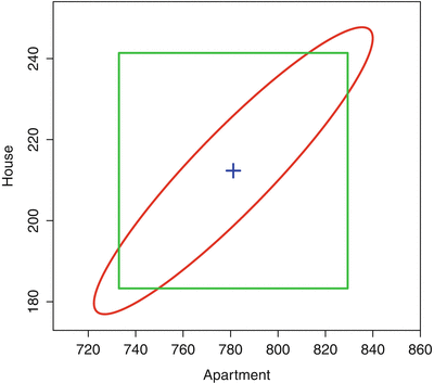
As an example of a multivariate statistical analysis, let us create a 95% joint (simultaneous) confidence interval of both the mean rent and housing prices.

Figure 1.1:

Joint 95% confidence ellipsoid for housing prices and monthly apartment rents. The box is formed from the marginal 95% confidence intervals. The sample averages are indicated in the center

The marginal confidence intervals treat each variable individually, and the resulting 95% confidence interval for the two means is pictured as a rectangle. The bivariate confidence ellipsoid takes into account the correlation between rents and housing prices resulting in an elongated elliptical shape oriented to reflect the positive correlation between these two prices.

The elliptical area and the rectangle overlap. There are also areas included in one figure but not the other. More importantly, notice the area of the ellipse is smaller than that of the rectangle. This difference in area illustrates the benefit of using multivariate methods over the marginal approach. If we were using univariate methods and obtaining confidence intervals for each variable individually, then the resulting confidence region is larger than the region that takes the bivariate relationship of rents and housing costs into account. This figure provides a graphical illustration of the benefits of using multivariate methods over the use of a series of univariate analyses.

1.2 Data Reduction or Structural Simplification

Which variables should be recorded when constructing a multivariate data set? We certainly want to include everything that might eventually turn out to be relevant, useful, and/or important. Much of these decisions require knowledge of the specific subject matter and cannot be adequately covered in a book on statistics. There is a trade-off between the fear of leaving out some information that later proves to be critical. Similarly, it may be next to impossible to go back to record data that was not recoded earlier.

Hopefully the subject matter experts have collected the most useful sets of measurements (with or without the aid of a statistician). The first task for the data analyst is to sort through it and determine those variables that are worthy of our attention. Similarly, much of the data collected may be redundant. A goal of data analysis is to sift through the data an identify what should be kept for further examination and what can safely be discarded.

Let us consider the data in Table The US is #17 on this list behind homogeneous populations of Finland, Korea, Hong Kong.

Table 1.2:

Reading and other academic scores from OECD nations

Reading subscales
Overall	Access	Integrate	Reflect
Nation	reading	retrieve	interpret	eval.	Continuous	Noncontin.	Math	Science
China:
Shanghai
Korea
Finland
Hong Kong
Peru
Azerbaijan
Kyrgyzstan

Source : OECD PISA 2009 database

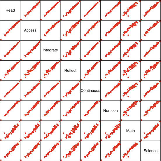
The overall reading score is broken down into five different subscales measuring specific skills. Mathematics and science are listed separately. How much is gained by providing the different subscales for reading? Is it possible to remove or combine some of these with little loss of detail?

More specifically, Fig.. The matrix scatterplot plots every pair of measurements against each other twice, with the axes reversed above and below the diagonal.

Next page

1234567...105

Light

Font size:

↓

↑

Georgia Tahoma Arial Verdana

Reset

Interval:

↓

↑

Bookmark:

Make

Similar books «Applied Multivariate Statistics with R»

Look at similar books to Applied Multivariate Statistics with R. We have selected literature similar in name and meaning in the hope of providing readers with more options to find new, interesting, not yet read works.

P. McCullagh

Tensor Methods in Statistics: Monographs on Statistics and Applied Probability

Steve Selbrede

The Statistics of Poker: Data Mining Statistics Applied to Small Stakes No Limit Holdem

David Doane

Applied Statistics Business Economics

Nickolay Trendafilov

Multivariate Data Analysis on Matrix Manifolds: (with Manopt)

Miah

Applied Statistics for Social and Management Sciences

Wolfgang Karl Härdle

Applied Multivariate Statistical Analysis

Eric Goh Ming Hui

2019

Janicak

Applied statistics in occupational safety and health

Keenan A. Pituch

Applied Multivariate Statistics for the Social Sciences: Analyses with SAS and IBMs SPSS

Seán Dineen

Multivariate Calculus and Geometry

Jussi Klemelä

Multivariate Nonparametric Regression and Visualization: With R and Applications to Finance

Geoffrey R. Norman

PDQ Statistics

Discussion, reviews of the book Applied Multivariate Statistics with R and just readers' own opinions. Leave your comments, write what you think about the work, its meaning or the main characters. Specify what exactly you liked and what you didn't like, and why you think so.