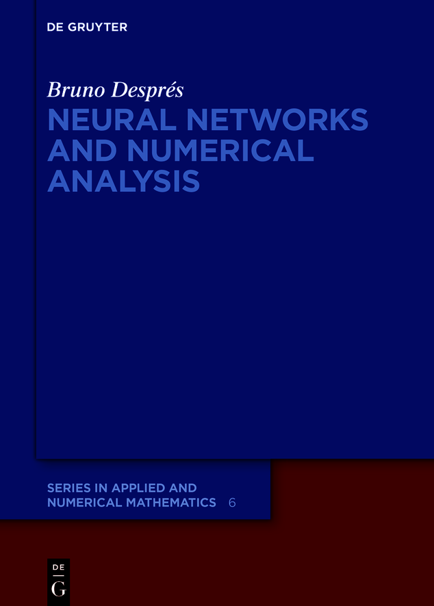
Bruno Després - Neural Networks and Numerical Analysis

De Gruyter Series in Applied and Numerical Mathematics

Edited by

Volume

ISBN 9783110783124

e-ISBN (PDF) 9783110783186

e-ISBN (EPUB) 9783110783261

Bibliographic information published by the Deutsche Nationalbibliothek

The Deutsche Nationalbibliothek lists this publication in the Deutsche Nationalbibliografie; detailed bibliographic data are available on the Internet at http://dnb.dnb.de.

2022 Walter de Gruyter GmbH, Berlin/Boston

Mathematics Subject Classification 2020: 68T07, 65Z05, 68T09, 65L99,

We share a philosophy about linear algebra: we think basis-free, we write basis-free, but when the chips are down we close the office door and compute with matrices like fury.

Irving Kaplansky

The basic problem is formulated in the context of interpolation of functions. Let fobj be an objective function modeling some problem of interest,

Let xi be an interpolation point in Rm . Let iRn denote a noise (small enough in a sense to be specified). Noise is an important notion for real data, because real measurements or real data are never perfect. Set

The pair (xi,yi)RmRn is called an interpolated data with noise iRn . If i=0 , then the interpolation data is noiseless.

The finite collection of interpolation data is the dataset

Starting from a given dataset D , a general question is implementing in a computer an approximation f of the objective function fobj . Some evident difficulties for the design of f are the level of the noise, the curse of dimension (that is, m and/or n take high values), the construction of good datasets (good datasets sample the objective function in meaningful regions), the fact that the implementation must be efficient for large N=#(D) , and the quality of the reconstructed function. Other aspects are developed in the notes.

At the end of the chapter, the structure of basic NNs is defined.

Standard linear algebra notations are used. For an arbitrary vector zRp in a space of arbitrary dimension p, we denote its square |z|2=i=1p|zi|20 . We have |z|2=z,z where the scalar product , is defined by

Let us consider two matrices M,NMmn(R) , two vectors a,bRm , and one vector cRn such that b=Mc . The contraction of matrices is denoted with equivalent notations

The tensorial product of two vectors is denoted ac=actMmn(R) . We have

A norm for matrices is defined as

which has the property ABAB .

Matrices with more than two axes of coefficients are called tensors. They will be introduced in Section on Convolutive Neural Networks.

A first ingredient is the least squares method. Consider a linear function f

where the parameters are represented by WMnm(R) , which is called the matrix of weights, and bRn , which is called the bias or the offset. Consider now the function

The space of parameters is Q=Mnm(R)Rn=Mn,m+1(R) . A way to minimize the difference between fobj encoded in the dataset D and the function f is determining the parameters that minimize J. That is, we consider an optimal value (W,b)Q in the sense of least squares: