Liviu Nicolaescu - An Invitation to Morse Theory

An Invitation to Morse Theory — read online for free the complete book (whole text) full work

Below is the text of the book, divided by pages. System saving the place of the last page read, allows you to conveniently read the book "An Invitation to Morse Theory" online for free, without having to search again every time where you left off. Put a bookmark, and you can go to the page where you finished reading at any time.

Light

Font size:

↓

↑

Georgia Tahoma Arial Verdana

Reset

Interval:

↓

↑

Bookmark:

Make

1234567...141

Liviu Nicolaescu Universitext An Invitation to Morse Theory 10.1007/978-1-4614-1105-5_1 Springer Science+Business Media, LLC 2012

1. Morse Functions

Liviu Nicolaescu 1

(1)

Department of Mathematics, University of Notre Dame, Notre Dame, USA

Liviu Nicolaescu

Email:

Abstract

In this first chapter, we introduce the reader to the main characters of our story, namely, the Morse functions, and we describe the properties which make them so useful. We describe their very special local structure (Morse lemma) and then we show that there are plenty of them around.

In this first chapter, we introduce the reader to the main characters of our story, namely, the Morse functions, and we describe the properties which make them so useful. We describe their very special local structure (Morse lemma) and then we show that there are plenty of them around.

1.1 The Local Structure of Morse Functions

Suppose that F : M N is a smooth (i.e., C ) map between smooth manifolds. The differential of F defines for every x M a linear map

Definition 1.1.

(a)

The point x M is called a critical point of F if

A point x M is called a regular point of F if it is not a critical point. The collection of all critical points of F is called the critical set of F and is denoted by { Cr } F .

(b)

The point y N is called a critical value of F if the fiber F 1( y ) contains a critical point of F . A point y N is called a regular value of F if it is not a critical value. The collection of all the critical values of F is called the discriminant set of F and is denoted by F .

(c)

A subset S N is said to be negligible if for every smooth open embedding , n =dim N , the preimage 1( S ) has Lebesgue measure zero in .

Theorem 1.2 (MorseSardFederer).

Suppose that M and N are smooth manifolds and F : M N is a smooth map. Then, the Hausdorff dimension of the discriminant set F is at most dim N 1. In particular, the discriminant set is negligible in N. Moreover, if F(M) has nonempty interior, then the set of regular values is dense in F(M).

For a proof, we refer to Federer [Fed, Theorem 3.4.3] or Milnor [M2].

Remark 1.3.

(a)

If M and N are real analytic manifolds and F is a proper real analytic map, then we can be more precise. The discriminant set is a locally finite union of real analytic submanifolds of N of dimensions less than dim N . Exercise 6.1 may perhaps explain why the set of critical values is called discriminant.

(b)

The range of a smooth map F : M N may have empty interior. For example, the range of the map , F ( x , y , z )=( x ,0), is the x -axis of the Cartesian plane . The discriminant set of this map coincides with the range.

Example 1.4.

Suppose is a smooth function. Then, x 0 M is a critical point of f if and only if .

Suppose M is embedded in an Euclidean space E and is a smooth function. Denote by f M the restriction of f to M . A point x 0 M is a critical point of f M if

This happens if either x 0 is a critical point of f , or and the tangent space to M at x 0 is contained in the tangent space at x 0 of the level set { f = f ( x 0)}. If f happens to be a nonzero linear function, then all its level sets are hyperplanes perpendicular to a fixed vector , and x 0 M is a critical point of f M if and only if , i.e., the hyperplane determined by f and passing through x 0 is tangent to M .

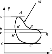
In Fig., we have depicted a smooth curve . The points A , B ,and C are critical points of the linear function f ( x , y )= y . The level sets of this function are horizontal lines and the critical points of its restriction to M are the points where the tangent space to the curve is horizontal. The points a , b ,and c on the vertical axis are critical values, while r is a regular value.

Example 1.5 ( Robot arms: critical configurations ).

We begin in this example the study of the critical points of a smooth function which arises in the design of robot arms. We will discuss only a special case of the problem when the motion of the arm is constrained to a plane. For slightly different presentations, we refer to the papers [Hau, KM, SV], which served as our sources of inspiration. The paper [Hau] discusses the most general version of this problem, when the motion of the arm is not necessarily constrained to a plane.

Fig. 1.1

The height function on a smooth curve in the plane

Fix positive real numbers r 1, , r n>0, n 2. A (planar) robot arm (or linkage) with n segments is a continuous curve in the Euclidean plane consisting of n line segments

of lengths

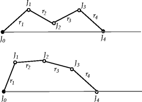
We will refer to the vertices J i as the joints of the robot arm. We assume that J 0 is fixed at the origin of the plane, and all the segments of the arm are allowed to rotate about the joints. Additionally, we require that the last joint be constrained to slide along the positive real semiaxis (see Fig.).

Fig. 1.2

A robot arm with four segments

A (robot arm) configuration is a possible position of the robot arm subject to the above constraints. Mathematically a configuration is described by an n -uple

Next page

1234567...141

Light

Font size:

↓

↑

Georgia Tahoma Arial Verdana

Reset

Interval:

↓

↑

Bookmark:

Make

Similar books «An Invitation to Morse Theory»

Look at similar books to An Invitation to Morse Theory. We have selected literature similar in name and meaning in the hope of providing readers with more options to find new, interesting, not yet read works.

Jeswant Gembali

Morse Code made Easy: Concepts

Herbert Morse

Where Do We Come From? Is Darwin Correct?: A Philosophical and Critical Study of Darwins Theory of “Natural Selection”

H. Morse (Henry Morse) Stephens

Revolutionary Europe, 1789-1815

Frederick Morse Cutler

The Old First Massachusetts Coast Artillery in War and Peace - the Original Classic Edition

J. J. Morse

Practical Occultism

Greg Morse

Railway Accidents

Edward S. Morse

Japanese Homes and Their Surroundings

Phil Morse [Morse

Rock The Dancefloor: The proven five-step formula for total DJing success

David Bishop

The Complete Inspector Morse

Jean-Claude Hausmann

Mod Two Homology and Cohomology

Michèle Audin Mihai Damian

Morse Theory and Floer Homology

Jackie Morse Kessler

Hunger

Discussion, reviews of the book An Invitation to Morse Theory and just readers' own opinions. Leave your comments, write what you think about the work, its meaning or the main characters. Specify what exactly you liked and what you didn't like, and why you think so.