Peter Shirley - Ray Tracing: The Rest Of Your Life

Ray Tracing: The Rest of Your Life

Peter Shirley

Copyright 2016 Peter Shirley. All rights reserved.

Chapter 0: Overview

In Ray Tracing In One Weekend and Ray Tracing: the Next Week , you built a real ray tracer.

In this volume, I assume you will be pursuing a career related to ray tracing and we will dive into the math of creating a very serious ray tracer. When you are done you should be ready to start messing with the many serious commercial ray tracers underlying the movie and product design industries. There are many many things I do not cover in this short volume; I dive into only one of many ways to write a Monte Carlo rendering program. I dont do shadow rays (instead I make rays more likely to go toward lights), bidirectional methods, Metropolis methods, or photon mapping. What I do is speak in the language of the field that studies those methods. I think of this book as a deep exposure that can be your first of many, and it will equip you with some of the concepts, math, and terms you will need to study the others.

As before, www.in1weekend.com will have further readings and references.

Acknowledgements: thanks to Dave Hart and Jean Buckley for help on the original manuscript. Thanks to Paul Melis and Matthew Heimlich for finding errors.

Chapter 1: A Simple Monte Carlo Program

Lets start with one of the simplest Monte Carlo (MC) programs. MC programs give a statistical estimate of an answer, and this estimate gets more and more accurate the longer you run it. This basic characteristic of simple programs producing noisy but ever-better answers is what MC is all about, and it is especially good for applications like graphics where great accuracy is not needed.

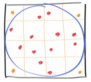
As an example, lets estimate Pi . There are many ways to do this, with the Buffon Needle problem being a classic case study. Well do a variation inspired by that. Suppose you have a circle inscribed inside a square:

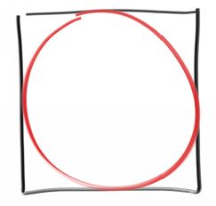
Now, suppose you pick random points inside the square. The fraction of those random points that end up inside the circle should be proportional to the area of the circle. The exact fraction should in fact be the ratio of the circle area to the square area.

Fraction = (Pi*R*R) / ((2R)*(2R)) = Pi/4

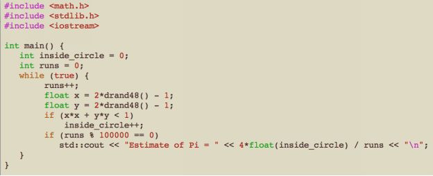
Since the R cancels out, we can pick whatever is computationally convenient. Lets go with R =1 centered at the origin:

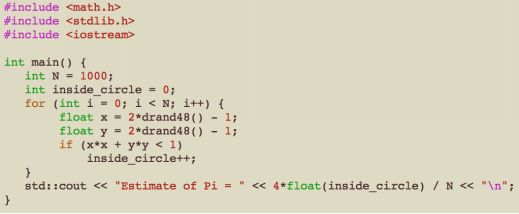
This gives me the answer Estimate of Pi = 3.196

If we change the program to run forever and just print out a running estimate:

We get very quickly near Pi, and then more slowly zero in on it. This is an example of the Law of Diminishing Returns , where each sample helps less than the last. This is the worst part of MC. We can mitigate this diminishing return by stratifying the samples (often called jittering ), where instead of taking random samples, we take a grid and take one sample within each:

This changes the sample generation, but we need to know how many samples we are taking in advance because we need to know the grid. Lets take a hundred million and try it both ways:

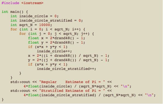
I get:

Regular Estimate of Pi = 3.1415

Stratified Estimate of Pi = 3.14159

Interestingly, the stratified method is not only better, it converges with a better asymptotic rate! Unfortunately, this advantage decreases with the dimension of the problem (so for example, with the 3D sphere volume version the gap would be less). This is called the Curse of Dimensionality . We are going to be very high dimensional (each reflection adds two dimensions), so I won't stratify in this book. But if you are ever doing single-reflection or shadowing or some strictly 2D problem, you definitely want to stratify.

Chapter 2: One Dimensional MC Integration

Integration is all about computing areas and volumes, so we could have framed Chapter 1 in an integral form if we wanted to make it maximally confusing. But sometimes integration is the most natural and clean way to formulate things. Rendering is often such a problem. Lets look at a classic integral:

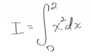
In computer sciency notation, we might write this as:

I = area( x^2, 0, 2 )

We could also write it as:

I = 2*average(x^2, 0, 2)

This suggests a MC approach:

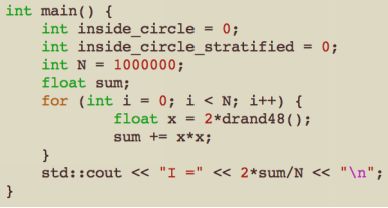
This, as expected, produces approximately the exact answer we get with algebra, I = 8/3 . But we could also do it for functions that we cant analytically integrate like log(sin(x)) . In graphics, we often have functions we can evaluate but cant write down explicitly, or functions we can only probabilistically evaluate. That is in fact what the ray tracing color() function of the last two books is-- we dont know what color is seen in every direction, but we can statistically estimate it in any given dimension.

One problem with the random program we wrote in the first two books is small light sources create too much noise because our uniform sampling doesnt sample the light often enough. We could lessen that problem if we sent more random samples toward the light, but then we would need to downweight those samples to adjust for the over-sampling. How we do that adjustment? To do that we will need the concept of a probability density function .

First, what is a density function ? Its just a continuous form of a histogram. Heres an example from the histogram Wikipedia page:

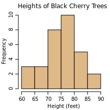
If we added data for more trees, the histogram would get taller. If we divided the data into more bins, it would get shorter. A discrete density function differs from a histogram in that it normalizes the frequency y-axis to a fraction or percentage (just a fraction times 100). A continuous histogram, where we take the number of bins to infinity, cant be a fraction because the height of all the bins would drop to zero. A density function is one where we take the bins and adjust them so they dont get shorter as we add more bins. For the case of the tree histogram above we might try:

Bin-height = (Fraction of trees between height H and H) / (H-H)

That would work! We could interpret that as a statistical predictor of a trees height:

Probability a random tree is between H and H = Bin-height*(H-H)

If we wanted to know about the chances of being in a span of multiple bins, we would sum.

A probability density function , henceforth pdf , is that fractional histogram made continuous.

Lets make a pdf and use it a bit to understand it more. Suppose I want a random number r between 0 and 2 whose probability is proportional to itself: r . We would expect the pdf p(r) to look something like the figure below. But how high should it be?