Daniel John Vogt - Soil and Plant Analysis for Forest Ecosystem Characterization

To illustrate the meanings of common statistical terms, a random set of 100 numbers (observations) was generated. This set comprises the population, and has the following parameters (as opposed to statistics, which concern samples taken from this population):

• population size, N = 100
• population mean, = 99 . 582
• population standard deviation, = 9 . 773
• population CV = 9 . 81%

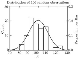
Frequency distribution of 100 normally distributed random observations, with mean = 99.582 and standard deviation = 9.773.

shows a frequency distribution of the population. Note that most of the values fall near the population mean, but a few are relatively far away. To be more precise, 68 values (68%) are within 1 of the mean, 95% are within 2, and 99.7% are within 3, meaning that 5% of the observations are more than 2 standard deviations away from the true population mean. So, if you make one observation on this population (i.e., take a random sample of 1), your estimate of the mean has a 68% probability of being within 9.773 of the true mean (i.e., no more than 9.81% off). Pretty good, huh? You might not want to bet the farm on your observation being right, though, because there is a 5% chance that you could be off by more than 2 9 . 773 = 19 . 546 (i.e., at least 19.63% off)!

The only way to be absolutely certain of (disregarding the likelihood of measurement errors) is to measure the entire population. Since this practice is usually out of the question, we typically take a sample of the population, and calculate various statistics (mean, and standard deviation, s ) to estimate the population parameters (true mean, , and standard deviation, ). As the sample size, n , gets larger (approaching N , the population size) we reduce (but cannot eliminate) the probability of error (sampling error).

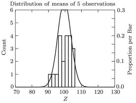
shows the distribution of 20 means of 5 observations each. Note that they are clustered much more tightly around the population mean.

Frequency distribution of 20 means of 5 observations each.

These 20 means have a mean of 99.582 (not surprisingly, its the same as the original population mean), and a standard deviation of 3.918substantially less than the original population standard deviation of 9.773. In fact, the population standard deviation, 9.773 divided by the square root of the sample size (5) equals 4.371, which is not too far from the observed value of 3.918. You may recognize the term S x as the standard error of the mean, which is an estimate of the standard deviation of a set of means, with n observations in each mean. In plain(er) English, any mean of 5 observations has a higher probability of being close to the true population mean than does any single observation ( n = 1). Such a mean is a sample from a population of all possible means of 5 observations; this population has a mean of = 99 . 582 (the same as the original population mean), and a standard deviation of the mean equal to S x = S/ (5) = 9 . 773 / 2 . 236 = 4 . 371, or the original standard deviation divided by the square root of the sample size. In practice, we dont know the population standard deviation. When we take our sample of size n, we estimate it by the sample standard deviation, divide by the square root of n, and use this standard error to calculate confidence intervals around our estimate of the mean.

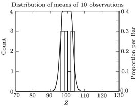
Similarly, we can take 10 samples of 10 observations each. The 10 means still have a mean of 99.582; the standard deviation is 2.337. The corresponding estimate is 3.090. The two numbers arent identical, because we only took 10 means of 10, a small sample of all possible means of 10. But you can see that the numbers calculated from this example approximate the theoretical values that the books say you should expect. shows the distribution of the means of 10.

Frequency distribution of 10 means of 10 observations each.

Analytical chemistry without QC is guesswork.

Introduction

Quality assurance (QA) is defined as a system of activities whose purpose is to provide to the producer or user of a product or service the assurance that it meets defined standards of quality with a stated level of confidence . In the context of a research project involving laboratory chemical analysis, a QA program will give you (the producer or the final user of the data) some confidence that the numbers you have generated are relatively free of errors due to sample contamination, instrument bias, etc., and will help you put limits on the uncertainty of your data.

Taylor further divides quality assurance into two components: quality control and quality assessment. Quality control (QC) refers to the routine practices carried out in all phases of the project (field sampling, sample storage and preparation, and laboratory work) to keep data quality in control, i.e., free (relatively speaking) from errors due to contamination, poor instrument calibration, loss of sample during transport and storage, etc. Such practices include use of distilled-deionized water and reagent-grade (or purer) chemicals, wearing gloves during sample handling, calibrating instruments daily, acid-rinsing glassware, etc. Quality assessment covers the tests that you perform to determine that you are, in fact, in control of quality, and includes such things as analyzing method blanks and Standard Reference Materials (SRMs) with each batch of samples, running calibration check samples periodically to verify that instrument calibration is stable, and taking part in inter-laboratory tests. Each sample collection, preparation, and analysis procedure will have its own QA/QC protocol. The use to which the data are going to be put will also determine the extent of the QA/QC steps required.

Appendix C Example Format for Field and Laboratory Data Sheets

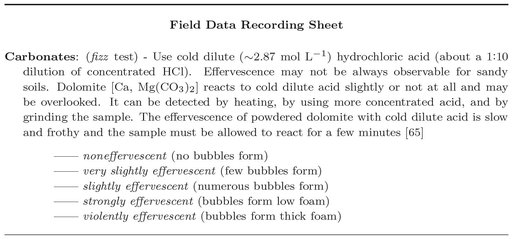
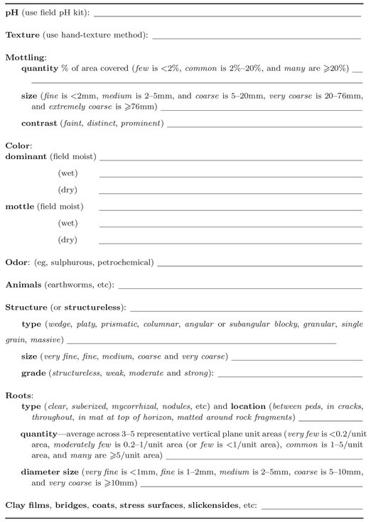
Example of a Field Data Recording Sheet.

Soil Data Summary Sheet.

Soil Data Summary
Soil ID code ___
Sand, % ___	Total CEC (cmol[+]/kg) ___
Silt, % ___	LOI % ___
Clay, % ___	Total carbon % ___
Textural class ___	Total nitrogen % ___