Benton - Orthogonal Functions: The Many Uses of

Orthogonal Functions: The Many Uses of — read online for free the complete book (whole text) full work

Below is the text of the book, divided by pages. System saving the place of the last page read, allows you to conveniently read the book "Orthogonal Functions: The Many Uses of" online for free, without having to search again every time where you left off. Put a bookmark, and you can go to the page where you finished reading at any time.

Light

Font size:

↓

↑

Georgia Tahoma Arial Verdana

Reset

Interval:

↓

↑

Bookmark:

Make

1234567...18

The Many Uses of

Orthogonal
Functions

by

D. James Benton

Copyright 2018 by D. James Benton, all rights reserved.

Foreword

Orthogonal functions are clever tools that unlock many mathematical puzzles. Once you've seen this done and understand how they work, you will find many more useful applications. This remarkable area of applied mathematics supports a wide range of technologies, ranging from CAT scans to satellite pictures from space to unraveling the sounds of the deep. Join me on a tour of this fascinating topic in which we will explore data sampling and approximation in both temporal and spatial dimensions.

All of the examples contained in this book,

(as well as a lot of free programs) are available at

http://www.dudleybenton.altervista.org/software/index.html

Programming

Most of the examples in this book are implemented in the C programming language. A few are implemented in VBA (Visual BASIC for Applications, or what Microsoft calls the language of Excel macros). BASIC stands for Beginner's All-Purpose Symbolic Instruction Code. If you're still using some form of BASIC and haven't yet graduated to a professional programming language, now is the time to do so and there is nothing better than C. It's in a class by itself.

examples\surface\surface.exe Hermite.tb2

examples\topography\transformed.p3d

examples\topography\inverse_distance.tb2

Table of Contents	page
Foreword	i
Programming	i
Chapter 1. Orthogonality: What Does it Mean?
Chapter 2. Magic of the Fast Fourier Transform
Chapter 3. Orthogonal Polynomials
Chapter 4. Infinite Domains
Chapter 5. 2D Data Applications
Chapter 6. Image Decomposition
Chapter 7. 3D Data Applications
Chapter 8: Spherical Data
Appendix A: Discrete Radon Transform
Appendix B. Image Rotation in Windows
Appendix C. Generation of Sinogram Images
Appendix D. Play It Anyway!
Appendix E: Triangle Gridder

Shepp-Logan Phantom

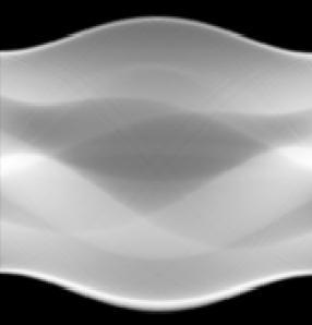
Corresponding Sinogram

Chapter 1. Orthogonality: What Does it Mean?

You must see this to appreciate it. While this may seem like a strange place to start, trust me, it will be eye opening Let's say you want to approximate some data using a simple polynomial of the form y=c+Cx+cx+cx+ The residual (i.e., error at each point) is given by:

(1.1)

In matrix form, R contains the r i , C contains the c i , X contains the x i , and Y contains the y i . We can write:

(1.2)

The sum of the squares of r i is equal to R T R , where R T is the transpose of R . Equation 1.2 can be expanded to obtain:

(1.3)

Equation 1.3 can be further expanded:

(1.4)

To find the coefficients resulting in the smallest residual, we take the derivative of Equation 1.4 with respect to C and set this equal to zero.

(1.5)

Solving Equation 1.5 for C yields:

(1.6)

This is the fundamental equation of linear regression seeking the least squares residual. Let's see how this works for a typical problem with four coefficients and a polynomial order of three. The spreadsheet (discrete.xls) can be found in the online archive in folder examples\discrete. The matrices are:

Because the number of constants equals the number of points in this case, the residual is zero. This seems straightforward enough and is easily implemented in Excel with functions TRANSPOSE(), MMULT(), and MINVERSE(), as illustrated in the spreadsheet. You will get the same result using LINEST(). Note that Excel's LINEST function returns the coefficients in reverse order. There's even a shorthand way of specifying the powers of X:

=TRANSPOSE(LINEST(U1:U4,B1:B4^{1,2,3},TRUE,FALSE))

We can set up a program (condition.c) to step through a range of orders to obtain the following table. There are several definitions of the condition number of a matrix, including the ratio of the largest to smallest singular value. We can estimate this important measure of stability by accumulating the product of the pivots. The larger the condition number, the more unstable the matrix, the more susceptible it is to round-off error, and the more meaningless the inverse.

n	condition
	82944
	1.19E+09
	6.19E+14
	1.57E+22
	2.56E+31
	3.36E+42
	2.35E+55
	1.26E+72
	4.45E+91
	7.78E+114
	3.95E+140

Next page

1234567...18

Light

Font size:

↓

↑

Georgia Tahoma Arial Verdana

Reset

Interval:

↓

↑

Bookmark:

Make

Similar books «Orthogonal Functions: The Many Uses of»

Look at similar books to Orthogonal Functions: The Many Uses of. We have selected literature similar in name and meaning in the hope of providing readers with more options to find new, interesting, not yet read works.

Paul Thurrott and Rafael Rivera

Windows 11 Field Guide

Frahaan Hussain

Learn OpenGL: Beginners guide to 3D rendering and game development with OpenGL and C++

Sergey Kosarevsky

3D Graphics Rendering Cookbook: A comprehensive guide to exploring rendering algorithms in modern OpenGL and Vulkan

Jayaram Prashanth

PowerShell 6.0 Linux Administration Cookbook: Over 150 recipes to leverage Microsofts open source automation framework and command line shell

Drake

Linux: 2019 Easy Guide for Beginners to Learn the Linux Operating System and Linux Command Line. 99 tips and tricks included

V. Scott Gordon

Computer Graphics Programming in OpenGL Using C++

David Wolff

OpenGL 4 Shading Language Cookbook

John Kessenich

OpenGL Programming Guide: The Official Guide to Learning OpenGL, Version 4.5 with SPIR-V

R. Stuart Ferguson

Practical Algorithms for 3D Computer Graphics

Prateek Mehta

Learn OpenGL ES: For Mobile Game and Graphics Development

Muhammad Mobeen Movania

OpenGL development cookbook

Harlan Carvey

Windows Forensic Analysis Toolkit, Third Edition: Advanced Analysis Techniques for Windows 7

Discussion, reviews of the book Orthogonal Functions: The Many Uses of and just readers' own opinions. Leave your comments, write what you think about the work, its meaning or the main characters. Specify what exactly you liked and what you didn't like, and why you think so.