Timo Heister - Scientific Computing: For Scientists and Engineers
Here you can read online Timo Heister - Scientific Computing: For Scientists and Engineers full text of the book (entire story) in english for free. Download pdf and epub, get meaning, cover and reviews about this ebook. City: Berlin, year: 2023, publisher: De Gruyter, genre: Computer. Description of the work, (preface) as well as reviews are available. Best literature library LitArk.com created for fans of good reading and offers a wide selection of genres:
Romance novel
Science fiction
Adventure
Detective
Science
History
Home and family
Prose
Art
Politics
Computer
Non-fiction
Religion
Business
Children
Humor
Choose a favorite category and find really read worthwhile books. Enjoy immersion in the world of imagination, feel the emotions of the characters or learn something new for yourself, make an fascinating discovery.

- Book:Scientific Computing: For Scientists and Engineers
- Author:
- Publisher:De Gruyter
- Genre:
- Year:2023
- City:Berlin
- Rating:5 / 5
- Favourites:Add to favourites
- Your mark:
Scientific Computing: For Scientists and Engineers: summary, description and annotation
We offer to read an annotation, description, summary or preface (depends on what the author of the book "Scientific Computing: For Scientists and Engineers" wrote himself). If you haven't found the necessary information about the book — write in the comments, we will try to find it.
Timo Heister: author's other books
Who wrote Scientific Computing: For Scientists and Engineers? Find out the surname, the name of the author of the book and a list of all author's works by series.


Scientific Computing: For Scientists and Engineers — read online for free the complete book (whole text) full work
Below is the text of the book, divided by pages. System saving the place of the last page read, allows you to conveniently read the book "Scientific Computing: For Scientists and Engineers" online for free, without having to search again every time where you left off. Put a bookmark, and you can go to the page where you finished reading at any time.
Font size:
Interval:
Bookmark:
The need to solve systems of linear equations arises across nearly all areas of engineering and science, business, statistics, economics, etc. In the chapters that follow, the need arises in numerical methods for solving boundary value differential equations and, in particular, in nonlinear equation solvers. We present in this chapter the method of Gaussian elimination to solve a system of linear equations with n equations and n unknowns. Gaussian elimination is an important first algorithm when learning about solving linear systems. For small, dense matrices (dense meaning mostly nonzero entries in the matrix), this algorithm and its variants are typically the best that can be done. However, for large sparse linear systems that arise from finite element/difference discretizations of differential equations, iterative solvers such as Conjugate Gradient and GMRES are typically better choices. We do not discuss such algorithms herein, but we refer the interested reader to the vast literature, in particular, the books Numerical Linear Algebra by Layton and Sussman (2014, Lulu publishing) and Numerical Linear Algebra by Trefethen and Bau (SIAM, 1995).
A linear equation of one variable takes the form
where a and b are given, and we want to determine the unknown value x. Solving this equation is easy, provided that a0 . If a=0 , then, however, there is no solution when b0 and infinitely many solutions when b=0 .
A linear system of two variables and two equations can be represented by
where the unknowns are x1 and x2 , and the other six numbers are given. Most college students have solved equations like this in high school, and most of the time a solution can be found by solving for one of the x in terms of the other from one equation, plugging that into the other equation to determine one of the x, then determining the remaining x using the known one. However, this procedure can fail: a solution need not exist, or there could also be infinitely many solutions, and in both these cases, this procedure will not produce a unique solution. Consider the following examples.
There are no solutions to the linear system
These equations are not consistent, and therefore no solution can exist.
There are infinitely many solutions to the linear system
Here the equations can be reduced to the same equation. Thus we have two unknowns, x1 and x2 , but only one equation. Thus any point on the line 2x1+x2=0 solves the system.
A geometric interpretation of solving linear systems is that if you were to plot each equation, the solution would be where they intersect. Hence, most often, two lines intersect at a point. However, the lines could be parallel and never intersect (this is the inconsistent case), or they could be the same line and intersect at every point on the line. The same idea can be extended to larger systems, and generally speaking, an n-equation, n-unknown consistent linear system will have a unique solution, provided that no equation is repeated.
In the 22 case, it is easy to see when an equation is repeated or inconsistent, but for larger systems, it is not always so easy. For example, consider the system of equations
Here the third equation is merely the sum of the first two equations. Hence it is not inconsistent, but it does not add anything to the system: if the first two equations are satisfied, then the third will automatically be satisfied. Two consistent equations with three unknowns means infinitely many solutions (two planes intersecting along a line).
It will be more convenient to use matrixvector notation to represent linear systems of equations. For example, the above 3-equation 3-unknown system can be equivalently written as
If we are going to try to use a numerical algorithm to find a solution to a system of equations, it would be nice to know up front whether or not a unique solution exists for a particular linear system. It turns out that there are many ways to determine this for small systems (say, n<10,000 ); for example, if the determinant of the matrix of coefficients is nonzero, then a solution exists and is unique. For larger systems, however, this determination can be very difficult. Fortunately, most linear systems that arise in science and engineering from common approaches such as finite element and finite difference methods are uniquely solvable, and if not, then often a mistake has been made in the derivation of the coefficients, or there is a different approach to the problem that would lead to a solvable system. Thus we will assume for the rest of this chapter that all the square linear systems have a unique solution, but we will keep in mind this potential problem when we analyze the algorithms. As the definition below states, this assumption can be made in several equivalent ways.
A square linear system Ax=b is uniquely solvable if the matrix A is nonsingular, which is equivalent to each of:
A is invertible;
det(A)0 ;
No eigenvalue of A is zero;
No singular value of A is zero;
The rows of A are linearly independent;
The columns of A are linearly independent.
A first step along the way to solving general linear systems of equations is solving triangular systems, which get their name because the matrix representation of their coefficients has only 0s either above or below the main diagonal (which goes from the top left to the bottom right). For such systems, finding solutions is straightforward, as we show in the following example.
We want to use back-substitution to solve the upper triangular system of equations
The last equation can be solved directly for x3 :
Plug in x3 into the first two equations and rewrite as a system of two equations:
Notice that the new, smaller 22 system remains upper triangular. That is a key point to the algorithm, as it can now be repeated over and over until the matrix reduces to a scalar. Solving the second equation directly for x2 gives x2=0 . Finally, plugging x2 into the first equation and solving yield x1=4 .
This procedure can easily be made into a general algorithm: For an nn upper triangular linear system starting at the bottom diagonal, solve for the unknown xn in that row, then plug it into the above rows. This leaves an (n1)(n1) triangular linear system, and so you repeat the process until the solution is determined. See for a visual representation of the following code that implements back-substitution:
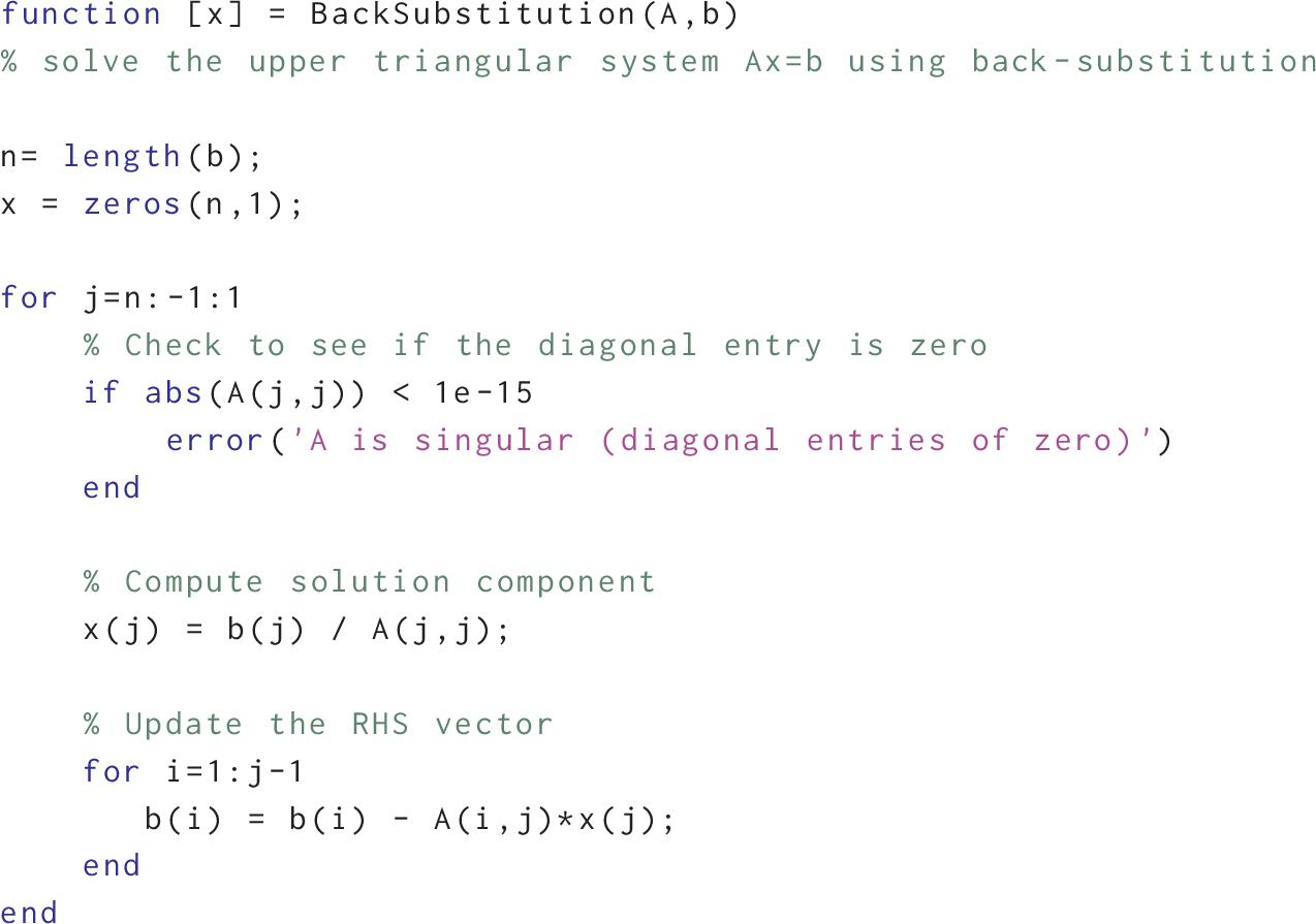
It can happen that this algorithm fails. If a diagonal entry is zero, then dividing by the diagonal entry is not possible. In such cases, it turns out that the rows of the matrix must have repetitions, which means there is not a unique solution to the problem it has either no solutions or infinitely many solutions. Note that the code above checks for this.
Font size:
Interval:
Bookmark:
Similar books «Scientific Computing: For Scientists and Engineers»
Look at similar books to Scientific Computing: For Scientists and Engineers. We have selected literature similar in name and meaning in the hope of providing readers with more options to find new, interesting, not yet read works.
Discussion, reviews of the book Scientific Computing: For Scientists and Engineers and just readers' own opinions. Leave your comments, write what you think about the work, its meaning or the main characters. Specify what exactly you liked and what you didn't like, and why you think so.