it-ebooks - TensorFlow Zero To All
Here you can read online it-ebooks - TensorFlow Zero To All full text of the book (entire story) in english for free. Download pdf and epub, get meaning, cover and reviews about this ebook. year: 2018, publisher: iBooker it-ebooks, genre: Romance novel. Description of the work, (preface) as well as reviews are available. Best literature library LitArk.com created for fans of good reading and offers a wide selection of genres:
Romance novel
Science fiction
Adventure
Detective
Science
History
Home and family
Prose
Art
Politics
Computer
Non-fiction
Religion
Business
Children
Humor
Choose a favorite category and find really read worthwhile books. Enjoy immersion in the world of imagination, feel the emotions of the characters or learn something new for yourself, make an fascinating discovery.
- Book:TensorFlow Zero To All
- Author:
- Publisher:iBooker it-ebooks
- Genre:
- Year:2018
- Rating:3 / 5
- Favourites:Add to favourites
- Your mark:
- 60
- 1
- 2
- 3
- 4
- 5
TensorFlow Zero To All: summary, description and annotation
We offer to read an annotation, description, summary or preface (depends on what the author of the book "TensorFlow Zero To All" wrote himself). If you haven't found the necessary information about the book — write in the comments, we will try to find it.
TensorFlow Zero To All — read online for free the complete book (whole text) full work
Below is the text of the book, divided by pages. System saving the place of the last page read, allows you to conveniently read the book "TensorFlow Zero To All" online for free, without having to search again every time where you left off. Put a bookmark, and you can go to the page where you finished reading at any time.
Font size:
Interval:
Bookmark:
- 1.1
- 1.2
- 1.3
- 1.4
- 1.5
- 1.6
- 1.7
- 1.8
- 1.9
- 1.10
- 1.11
- 1.12
- 1.13
- 1.14
- 1.15
- 1.16
- 1.17
- 1.18
- 1.19
- 1.20
- 1.21
- 1.22
- 1.23
- 1.24
- 1.25
- 1.26
- 1.27
- 1.28
- 1.29
- 1.30
- 1.31
- 1.32
- 1.33
- 1.34
- 1.35
- 1.36
- 1.37
- 1.38
- 1.39
- 1.40
- 1.41
- 1.42
- 1.43
- 1.44
- 1.45
- 1.46
- 1.47
- 1.48
- 1.49
- 1.50
- 1.51
- 1.52
- 1.53
- 1.54
- 1.55
From: hunkim/DeepLearningZeroToAll
Author: hunkim
https://www.tensorflow.org/get_started/get_started
import tensorflow as tftf.__version__'1.0.0'# Create a constant op # This op is added as a node to the default graph hello = tf.constant( "Hello, TensorFlow!" ) # start a TF session sess = tf.Session() # run the op and get result print(sess.run(hello))b'Hello, TensorFlow!'# a rank 0 tensor; this is a scalar with shape [] [ ,, ] # a rank 1 tensor; this is a vector with shape [3] [[, , ], [, , ]] # a rank 2 tensor; a matrix with shape [2, 3] [[[, , ]], [[, , ]]] # a rank 3 tensor with shape [2, 1, 3][[[1.0, 2.0, 3.0]], [[7.0, 8.0, 9.0]]]node1 = tf.constant( 3.0 , tf.float32)node2 = tf.constant( 4.0 ) # also tf.float32 implicitly node3 = tf.add(node1, node2)print( "node1:" , node1, "node2:" , node2)print( "node3: " , node3)node1: Tensor("Const_1:0", shape=(), dtype=float32) node2: Tensor("Const_2:0", shape=(), dtype=float32)node3: Tensor("Add:0", shape=(), dtype=float32)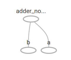
sess = tf.Session()print( "sess.run(node1, node2): " , sess.run([node1, node2]))print( "sess.run(node3): " , sess.run(node3))sess.run(node1, node2): [3.0, 4.0]sess.run(node3): 7.0a = tf.placeholder(tf.float32)b = tf.placeholder(tf.float32)adder_node = a + b # + provides a shortcut for tf.add(a, b) print(sess.run(adder_node, feed_dict={a: , b: 4.5 }))print(sess.run(adder_node, feed_dict={a: [,], b: [, ]}))7.5[ 3. 7.]add_and_triple = adder_node * print(sess.run(add_and_triple, feed_dict={a: , b: 4.5 }))22.5# Lab 2 Linear Regression import tensorflow as tftf.set_random_seed() # for reproducibility # X and Y data x_train = [, , ]y_train = [, , ] # Try to find values for W and b to compute y_data = x_data * W + b # We know that W should be 1 and b should be 0 # But let TensorFlow figure it out W = tf.Variable(tf.random_normal([]), name= 'weight' )b = tf.Variable(tf.random_normal([]), name= 'bias' ) # Our hypothesis XW+b hypothesis = x_train * W + b # cost/loss function cost = tf.reduce_mean(tf.square(hypothesis - y_train)) # Minimize optimizer = tf.train.GradientDescentOptimizer(learning_rate= 0.01 )train = optimizer.minimize(cost) # Launch the graph in a session. sess = tf.Session() # Initializes global variables in the graph. sess.run(tf.global_variables_initializer()) # Fit the line for step in range( 2001 ): sess.run(train) if step % == : print(step, sess.run(cost), sess.run(W), sess.run(b)) # Learns best fit W:[ 1.], b:[ 0.] '''0 2.82329 [ 2.12867713] [-0.85235667]20 0.190351 [ 1.53392804] [-1.05059612]40 0.151357 [ 1.45725465] [-1.02391243]...1920 1.77484e-05 [ 1.00489295] [-0.01112291]1940 1.61197e-05 [ 1.00466311] [-0.01060018]1960 1.46397e-05 [ 1.004444] [-0.01010205]1980 1.32962e-05 [ 1.00423515] [-0.00962736]2000 1.20761e-05 [ 1.00403607] [-0.00917497]'''# Lab 2 Linear Regression import tensorflow as tftf.set_random_seed() # for reproducibility # Try to find values for W and b to compute y_data = W * x_data + b # We know that W should be 1 and b should be 0 # But let's use TensorFlow to figure it out W = tf.Variable(tf.random_normal([]), name= 'weight' )b = tf.Variable(tf.random_normal([]), name= 'bias' ) # Now we can use X and Y in place of x_data and y_data # # placeholders for a tensor that will be always fed using feed_dict # See http://stackoverflow.com/questions/36693740/ X = tf.placeholder(tf.float32, shape=[ None ])Y = tf.placeholder(tf.float32, shape=[ None ]) # Our hypothesis XW+b hypothesis = X * W + b # cost/loss function cost = tf.reduce_mean(tf.square(hypothesis - Y)) # Minimize optimizer = tf.train.GradientDescentOptimizer(learning_rate= 0.01 )train = optimizer.minimize(cost) # Launch the graph in a session. sess = tf.Session() # Initializes global variables in the graph. sess.run(tf.global_variables_initializer()) # Fit the line for step in range( 2001 ): cost_val, W_val, b_val, _ = \ sess.run([cost, W, b, train], feed_dict={X: [, , ], Y: [, , ]}) if step % == : print(step, cost_val, W_val, b_val) # Learns best fit W:[ 1.], b:[ 0] '''...1980 1.32962e-05 [ 1.00423515] [-0.00962736]2000 1.20761e-05 [ 1.00403607] [-0.00917497]''' # Testing our model print(sess.run(hypothesis, feed_dict={X: []}))print(sess.run(hypothesis, feed_dict={X: [ 2.5 ]}))print(sess.run(hypothesis, feed_dict={X: [ 1.5 , 3.5 ]})) '''[ 5.0110054][ 2.50091505][ 1.49687922 3.50495124]''' # Fit the line with new training data for step in range( 2001 ): cost_val, W_val, b_val, _ = \ sess.run([cost, W, b, train], feed_dict={X: [, , , , ], Y: [ 2.1 , 3.1 , 4.1 , 5.1 , 6.1 ]}) if step % == : print(step, cost_val, W_val, b_val) # Testing our model print(sess.run(hypothesis, feed_dict={X: []}))print(sess.run(hypothesis, feed_dict={X: [ 2.5 ]}))print(sess.run(hypothesis, feed_dict={X: [ 1.5 , 3.5 ]})) '''1960 3.32396e-07 [ 1.00037301] [ 1.09865296]1980 2.90429e-07 [ 1.00034881] [ 1.09874094]2000 2.5373e-07 [ 1.00032604] [ 1.09882331][ 6.10045338][ 3.59963846][ 2.59931231 4.59996414]'''# From https://www.tensorflow.org/get_started/get_started import tensorflow as tf # Model parameters W = tf.Variable([ .3 ], tf.float32)b = tf.Variable([ -.3 ], tf.float32) # Model input and output x = tf.placeholder(tf.float32)y = tf.placeholder(tf.float32)linear_model = x * W + b # cost/loss function loss = tf.reduce_sum(tf.square(linear_model - y)) # sum of the squares # optimizer optimizer = tf.train.GradientDescentOptimizer( 0.01 )train = optimizer.minimize(loss) # training data x_train = [, , , ]y_train = [, -1 , -2 , -3 ] # training loop init = tf.global_variables_initializer()sess = tf.Session()sess.run(init) # reset values to wrong for i in range( 1000 ): sess.run(train, {x: x_train, y: y_train}) # evaluate training accuracy curr_W, curr_b, curr_loss = sess.run([W, b, loss], {x: x_train, y: y_train})print( "W: %s b: %s loss: %s" % (curr_W, curr_b, curr_loss))# Lab 3 Minimizing Cost import tensorflow as tf import matplotlib.pyplot as plttf.set_random_seed() # for reproducibility X = [, , ]Y = [, , ]W = tf.placeholder(tf.float32) # Our hypothesis for linear model X * W hypothesis = X * W # cost/loss function cost = tf.reduce_mean(tf.square(hypothesis - Y)) # Launch the graph in a session. sess = tf.Session() # Variables for plotting cost function W_history = []cost_history = [] for i in range( -30 , ): curr_W = i * 0.1 curr_cost = sess.run(cost, feed_dict={W: curr_W}) W_history.append(curr_W) cost_history.append(curr_cost) # Show the cost function plt.plot(W_history, cost_history)plt.show()Font size:
Interval:
Bookmark:
Similar books «TensorFlow Zero To All»
Look at similar books to TensorFlow Zero To All. We have selected literature similar in name and meaning in the hope of providing readers with more options to find new, interesting, not yet read works.
Discussion, reviews of the book TensorFlow Zero To All and just readers' own opinions. Leave your comments, write what you think about the work, its meaning or the main characters. Specify what exactly you liked and what you didn't like, and why you think so.


