it-ebooks - Deep Learning with Keras and Tensorflow

Deep learning allows computational models that are composed of multiple processing layers to learn representations of data with multiple levels of abstraction.

These methods have dramatically improved the state-of-the-art in speech recognition, visual object recognition, object detection and many other domains such as drug discovery and genomics.

Deep learning is one of the leading tools in data analysis these days and one of the most common frameworks for deep learning is Keras.

The Tutorial will provide an introduction to deep learning using keras with practical code examples.

• Getting a conceptual understanding of multi-layer neural networks
• Training neural networks for image classification
• Implementing the powerful backpropagation algorithm
• Debugging neural network implementations

In machine learning and cognitive science, an artificial neural network (ANN) is a network inspired by biological neural networks which are used to estimate or approximate functions that can depend on a large number of inputs that are generally unknown

An ANN is built from nodes (neurons) stacked in layers between the feature vector and the target vector.

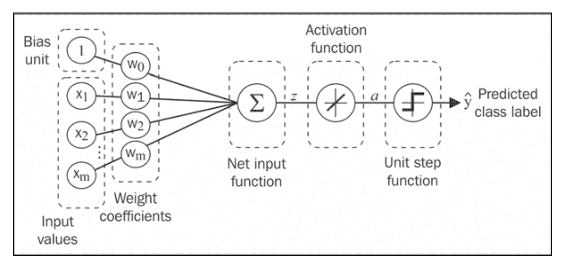
A node in a neural network is built from Weights and Activation function

An early version of ANN built from one node was called the Perceptron

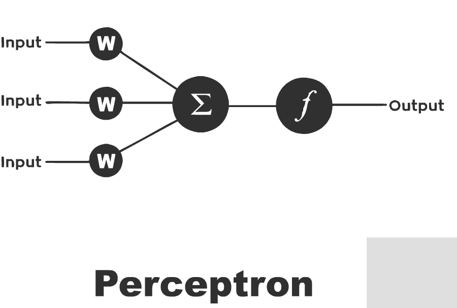
The Perceptron is an algorithm for supervised learning of binary classifiers. functions that can decide whether an input (represented by a vector of numbers) belongs to one class or another.

Much like logistic regression, the weights in a neural net are being multiplied by the input vertor summed up and feeded into the activation function's input.

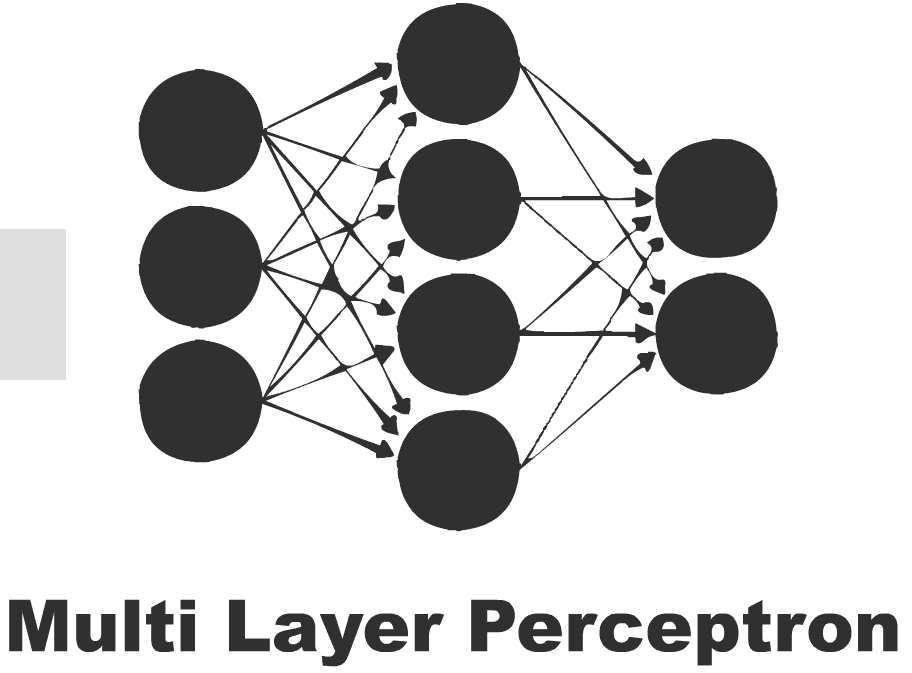
A Perceptron Network can be designed to have multiple layers, leading to the Multi-Layer Perceptron (aka MLP)

(Source: Python Machine Learning, S. Raschka)

• We use a gradient descent optimization algorithm to learn the Weights Coefficients of the model.
  
• In every epoch (pass over the training set), we update the weight vector $w$ using the following update rule:

$$w = w + \Delta w, \text{where } \Delta w = - \eta \nabla J(w)

$$

In other words, we computed the gradient based on the whole training set and updated the weights of the model by taking a step into the opposite direction of the gradient $ \nabla J(w)$.

In order to fin the optimal weights of the model, we optimized an objective function (e.g. the Sum of Squared Errors (SSE)) cost function $J(w)$.

Furthermore, we multiply the gradient by a factor, the learning rate $\eta$ , which we choose carefully to balance the speed of learning against the risk of overshooting the global minimum of the cost function.

In gradient descent optimization, we update all the weights simultaneously after each epoch, and we define the partial derivative for each weight $w_j$ in the weight vector $w$ as follows:

$$\frac{\partial}{\partial wj} J(w) = \sum{i} ( y^{(i)} - a^{(i)} ) x^{(i)}_j

$$

Note: The superscript $(i)$ refers to the i-th sample. The subscript $j$ refers to the j-th dimension/feature

Here $y^{(i)}$ is the target class label of a particular sample $x^{(i)}$ , and $a^{(i)}$ is the activation of the neuron

(which is a linear function in the special case of Perceptron).

We define the activation function $\phi(\cdot)$ as follows:

$$\phi(z) = z = a = \sum_{j} w_j x_j = \mathbf{w}^T \mathbf{x}

$$

While we used the activation $\phi(z)$ to compute the gradient update, we may use a threshold function(Heaviside function) to squash the continuous-valued output into binary class labels for prediction:

$$\hat{y} = \begin{cases} 1 & \text{if } \phi(z) \geq 0 \ 0 & \text{otherwise}\end{cases}

$$

We will build the neural networks from first principles. We will create a very simple model and understand how it works. We will also be implementing backpropagation algorithm.

Please note that this code is not optimized and not to be used in production.

This is for instructive purpose - for us to understand how ANN works.

Libraries like theano have highly optimized code.

Take a look at this notebook :

If you want a sneak peek of alternate (production ready) implementation of Perceptron for instance try:

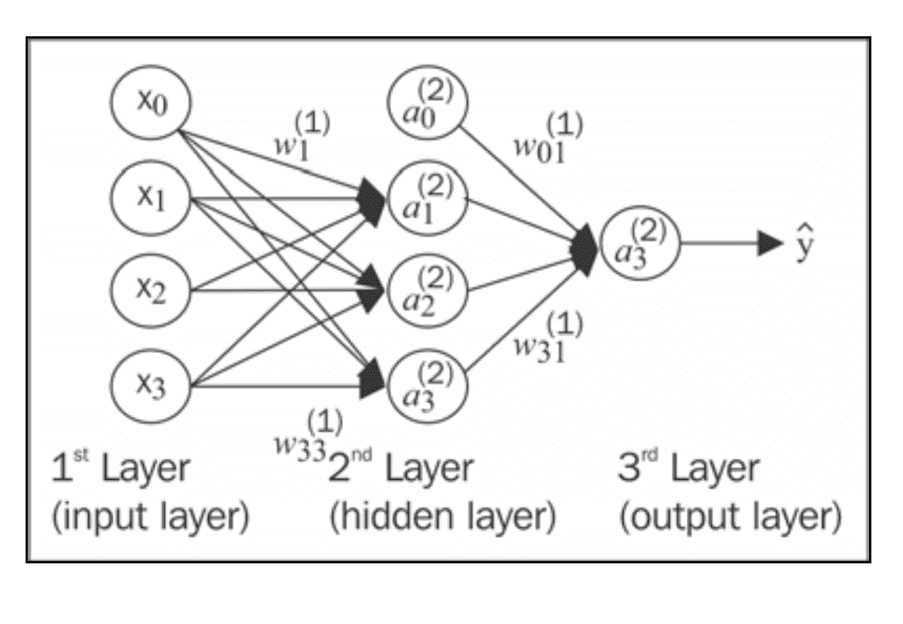
(Source: Python Machine Learning, S. Raschka)

Now we will see how to connect multiple single neurons to a multi-layer feedforward neural network; this special type of network is also called a multi-layer perceptron (MLP).

The figure shows the concept of an MLP consisting of three layers: one input layer, one hidden layer, and one output layer.

The units in the hidden layer are fully connected to the input layer, and the output layer is fully connected to the hidden layer, respectively.

If such a network has more than one hidden layer, we also call it a deep artificial neural network.

we denote the ith activation unit in the lth layer as $ai^{(l)}$ , and the activation units $a_0^{(1)}$ and $a_0^{(2)}$ are the bias units, respectively, which we set equal to $1$.
The _activation of the units in the input layer is just its input plus the bias unit:

$$\mathbf{a}^{(1)} = [a_0^{(1)}, a_1^{(1)}, \ldots, a_m^{(1)}]^T = [1, x_1^{(i)}, \ldots, x_m^{(i)}]^T

$$
Note: $x_j^{(i)}$ refers to the jth feature/dimension of the ith sample

The terminology around the indices (subscripts and superscripts) may look a little bit confusing at first.

You may wonder why we wrote $w{j,k}^{(l)}$ and not $w{k,j}^{(l)}$ to refer to the weight coefficient that connects the kth unit in layer $l$ to the jth unit in layer $l+1$.

What may seem a little bit quirky at first will make much more sense later when we vectorize