Lopez C.P. - Linear Algebra with Mathematica

Mathematica enables correct work withthis type of functions, which are defined, in the majority of cases, relying onthe conditional commands, as If, Which, etc. In Mathematica functions suchflooring defined cablul especially operator condicuionla If using adoptsthe following syntax: If[condition, expression1, expression2] Whenthe condition is true evaluates expression1, and when false expression2 isevaluated. As an application example we define the function: In[12]:=Delta[x_] := If [x==0, 1, 0] Thisfunction is set to 1 if x = 0 and in any other case, 0. Wethen define the following function: In[13]: = f [x_]: = If [x > 0, 1, 0] Thisfunction takes the value 1 for all x greater than 0, and takes the value 0 forall x less than or equal to 0. Tographically represent this function, we propose: In[14]:=Plot [f[x], {x, -1, 1}, Axes->{0, 0.5}]Out [14] =see Figure 2.1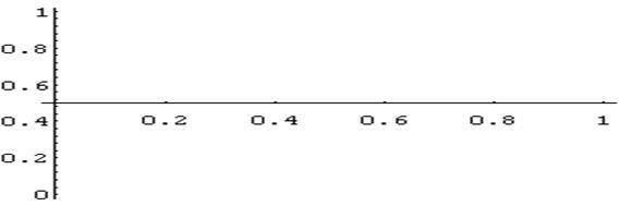 Figure 2.1 Whenit is necessary to control the function, rather than across a single condition,but of several, is available the operator condicuional Wich with thefollowing syntax: Which[condition1, expression1,..., conditionn, expressionn] Ifthe conditioni is true the expressioni is evaluated (i=1, 2, ,n).Putting True as the last condition, gets evaluate the last expression if noneof the previous conditions have been certain. Asan example we consider the piecewise-defined function look: In[15]:=g[x_]:=Which[-2<=x<=2,x^2, -3<=-3, 0, 2<=x, 0, True,x^2] Thefunction g to pieces at intervals is defined (- , - 3) (- 3, - 2), (- 2.2), (2.3), (3, ). Wecan graphically represent the function g as follows: In[16]: = Plot [g [x], {x, - 4, 4}]Out[16] = see Figure 2.2 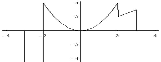Figure 2.2 Alsowe can graphically represent the function for the function g as follows: In[16]:=Plot[g'[x], {x, -4, 4}] Wewill now define a function, called rect, which is set to 1 in the interval[-1/3, 1/3] and which is worth $ 0 in the rest of the real line. In[23]:=rect[x_] := 1 /. (-1/3 <= x && x <= 1/3)In[24]:=rect[x_] := 0 /. (-1/3 <= x && x <= 1/3)In[24]:=rect[x_] := 0 /.

Abs[x] > 1/3 Thisfunction can also be written in the following way: In[22]:= Clear[rect];In[23]:= rect[x_ /. (-1/3 <= x && x >= 1/3)] := 1In[24]:= rect[x_ /. Abs[x] > 1/3] := 0