David Borthwick - Introduction to Partial Differential Equations

Introduction to Partial Differential Equations — read online for free the complete book (whole text) full work

Below is the text of the book, divided by pages. System saving the place of the last page read, allows you to conveniently read the book "Introduction to Partial Differential Equations" online for free, without having to search again every time where you left off. Put a bookmark, and you can go to the page where you finished reading at any time.

Light

Font size:

↓

↑

Georgia Tahoma Arial Verdana

Reset

Interval:

↓

↑

Bookmark:

Make

1234567...137

Springer International Publishing AG 2016

David Borthwick Introduction to Partial Differential Equations Universitext 10.1007/978-3-319-48936-0_1

1. Introduction

David Borthwick 1

(1)

Department of Mathematics and Computer Science, Emory University, Atlanta, GA, USA

David Borthwick

Email:

1.1 Partial Differential Equations

Continuous phenomena, such as wave propagation or fluid flow, are generally modeled with partial differential equations (PDE), which express relationships between rates of change with respect to multiple independent variables. In contrast, phenomena that can be described with a single independent variable, such as the motion of a rigid body in classical physics, are modeled by ordinary differential equations (ODE).

A general PDE for a function u has the form

(1.1)

The order of this equation is m , the order of the highest derivative appearing (which is assumed to be finite). A classical solution u admits continuous partial derivatives up to order m and satisfies () at all points in its domain. In certain situations the differentiability requirements can be relaxed, allowing us to define weak solutions that do not solve the equation literally.

A somewhat subtle aspect of the definition () is the fact that the equation is required to be local . This means that functions and derivatives appearing in the equation are all evaluated at the same point.

Although classical physics provided the original impetus for the development of PDE theory, PDE models have since played a crucial role in many other fields, including engineering, chemistry, biology, ecology, medicine, and finance. Many industrial applications of mathematics are based on the numerical analysis of PDE.

Most PDE are not solvable in the explicit sense that a simple calculus problem can be solved. That is, we typically cannot obtain a exact formula for . Therefore much of the analysis of PDE is focused on drawing meaningful conclusions from an equation without actually writing down a solution.

1.2 Example: dAlemberts Wave Equation

One of the earliest and most influential PDE models was the wave equation , developed by Jean dAlembert in 1746 to describe the motion of a vibrating string. With physical constants normalized to 1, the equation reads

(1.2)

where u ( t , x ) denotes the vertical displacement of the string at position x and time t . If the string has length and is attached at both ends, then we also require that for all t . We will discuss the formulation of this model in Sect..

DAlembert also found a general formula for the solution of () is solved by any function of the form , assuming f is twice-differentiable. Given two such functions on , we can write a general solution

(1.3)

A similar formula applies in the case of a string with fixed ends. If f is -periodic on , meaning for all x , then it is easy to check that

(1.4)

satisfies for any t .

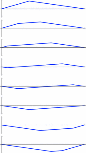
One curious feature of this formula is that it appears to give a sensible solution even in cases where f is not differentiable. For example, to model a plucked string we might take the initial displacement to be a simple piecewise linear function in the form of a triangle from the fixed endpoints, as shown in Fig..

Fig. 1.1

Initial state of a plucked string

If we extend this to an odd, -periodic function on , then the formula (. The initial kink splits into two kinks which travel in opposite directions on the string and and appear to rebound from the fixed ends.

Fig. 1.2

Evolution of the plucked string, starting from at the top

This is not a classical solution because u is not differentiable at the kinks. However, u does satisfy the requirements for a weak solution, as we will see in Chap..

Although a physical string could not exhibit sharp corners without breaking, the piecewise linear solutions are nevertheless physically reasonable. Direct observations of plucked and bowed strings were first made in the late 19th century by Hermann von Helmholtz, who saw patterns of oscillation quite similar to what is shown in Fig.. The appearance of kinks propagating along the string is striking, although the corners are not exactly sharp.

1.3 Types of Equations

There is no general theory of PDE that allows us to analyze all equations of the form (). To make progress it is necessary to restrict our attention to certain classes of equations and develop methods appropriate to those.

The most fundamental distinction between PDE is the property of linearity . A PDE is called linear if it can be written in the form

(1.5)

where f is some function independent of u , and L is a differential operator. Many of the important classical PDE that we will discuss in this book are linear and of first or second order. For such cases L has the general form

Next page

1234567...137

Light

Font size:

↓

↑

Georgia Tahoma Arial Verdana

Reset

Interval:

↓

↑

Bookmark:

Make

Similar books «Introduction to Partial Differential Equations»

Look at similar books to Introduction to Partial Differential Equations. We have selected literature similar in name and meaning in the hope of providing readers with more options to find new, interesting, not yet read works.

Nakhle H. Asmar

Partial differential equations with fourier series and boundary value problems : third edition

Jeremy Gray

Change and Variations: A History of Differential Equations to 1900

Allan Struthers

Differential Equations: For Scientists and Engineers

Hillen Thomas

Partial Differential Equations: Theory and Completely Solved Problems

Michael E. Taylor

Partial differential equations. II, Qualitative studies of linear equations

Jost

Partial Differential Equations

Karline Soetaert

Solving Differential Equations in R

Stanley J. Farlow

Partial Differential Equations for Scientists and Engineers

Stanley J. Farlow

An Introduction to Differential Equations and Their Applications

Dorina Mitrea

Distributions, Partial Differential Equations, and Harmonic Analysis

Carroll

Abstract Methods in Partial Differential Equations

Lennart Edsberg

Introduction to Computation and Modeling for Differential Equations

Discussion, reviews of the book Introduction to Partial Differential Equations and just readers' own opinions. Leave your comments, write what you think about the work, its meaning or the main characters. Specify what exactly you liked and what you didn't like, and why you think so.