Many important ideas in mathematics are developed within the framework of physical science, and mathematical equations, especially partial differential equations, provides the language to formulate these ideas. In reverse, advances in mathematics provides the stimulus for new advancements in science. Over the years mathematicians and scientists extended these methodologies to include nearly all areas of science and technology, and a paradigm emerged called mathematical modeling. A mathematical model is an equation, or set of equations, whose solution describes the physical behavior of the related physical system. In this context we say, for example, that Maxwells equations form a model for electromagnetic phenomena. Like most mathematical models, Maxwells equations are based on physical observations. But the model is so accurate, we regard the model itself as describing an actual physical law. Other models, for example a model of how a disease spreads in a population, are more conceptual. Such models often explain observations, but only in a highly limited sense. In general, a mathematical model is a simplified description, or caricature, of reality expressed in mathematical terms. Mathematical modeling involves observation, selection of relevant physical variables, formulation of the equations, analysis of the equations and simulation, and, finally, validation of the model to ascertain whether indeed it is predictive. The subject of partial differential equations encompasses all types of models, from physical laws like Maxwells equations in electrodynamics, to conceptual laws that describe the spread of an plant invasive species on a savanna.
1.1 PDE Models
In this book we examine models that can be described by partial differential equations. The focus is on the origin of such models and tools used for their analysis. Of particular interest are models in diffusion and heat flow, wave propagation, and transport of energy, chemicals, and other matter. It is impossible to overestimate the role and importance of PDEs in science and engineering.
Readers should be familiar with systems governed by ordinary differential equations (ODEs). For example, a typical ODE model in population ecology is the logistic model
which is a simple equation for population growth where the per capita rate of change of population,

, is a decreasing function of the population. Here t is time, and

is the population of a given system of individuals. We refer to u as the state and say that the evolution of the state variable is governed by the model equation. The positive numbers r and K are given physical parameters that represent the relative growth rate and carrying capacity, respectively; presumably, r and K can be measured for the population under investigation. The solution to the logistic equation is easily found by separation of variables to be
where

is the initial population. The logistic model accurately describes some populations having a sigmoid growth shape. In general, an ODE model has the form
where F is a given functional relation between t , u , and m parameters

. Often the model includes an initial condition of the form

, where u 0 is a given state value at t =0. More generally, an ODE model may consist of a system of n ODEs for n state variables

A PDE model differs from an ODE model in that the state variable u depends on more than one independent variable. ODEs govern the evolution of a system in time, and observations are made in time. PDEs model the evolution of a system in both time and space; the system can be observed both in a time interval and in a spatial region (which may be one-, two-, or three-dimensional). PDE models may also be independent of time, but depend on several spatial variables. Two examples of PDEs are
The wave equation describes the propagation of waves in a one dimensional medium. The unknown function

is a function of position x and time t . In Laplaces equation, the unknown state is a function

, where x and y are spatial variables. It models, for example, equilibrium temperatures in a two-dimensional region of the plane with prescribed temperatures on its boundary.
Example 1.1
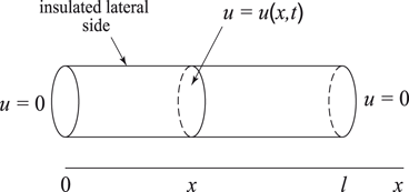
( Heat flow ) Consider the problem of determining the temperature in a thin, laterally insulated, cylindrical, metal bar of length l and unit cross-sectional area, whose two ends are maintained at a constant zero degrees, and whose temperature initially (at time zero) varies along the bar and is given by a fixed function

. See Figure .
Figure 1.1
A laterally insulated metal bar with zero temperature at both ends. Heat flows in the axial, or x -direction, and

is the temperature of the cross-section at x at time t . At time t =0 the temperature at locations x is given by

How does the bar cool down? In this case, the state variable u is the temperature, and it depends upon both when the measurement is taken and where in the bar it is taken. Thus,







 , is a decreasing function of the population. Here t is time, and
  is the population of a given system of individuals. We refer to u as the state and say that the evolution of the state variable is governed by the model equation. The positive numbers r and K are given physical parameters that represent the relative growth rate and carrying capacity, respectively; presumably, r and K can be measured for the population under investigation. The solution to the logistic equation is easily found by separation of variables to be
 is the initial population. The logistic model accurately describes some populations having a sigmoid growth shape. In general, an ODE model has the form
 . Often the model includes an initial condition of the form
  , where u 0 is a given state value at t =0. More generally, an ODE model may consist of a system of n ODEs for n state variables

 is a function of position x and time t . In Laplaces equation, the unknown state is a function
  , where x and y are spatial variables. It models, for example, equilibrium temperatures in a two-dimensional region of the plane with prescribed temperatures on its boundary.
 . See Figure .
 is the temperature of the cross-section at x at time t . At time t =0 the temperature at locations x is given by
