Linear Algebra Coding with Python
Author
The author studied at Seoul National University (Ph.D.) and currently serves as the director of Nnode LTD. He is interested in analyzing data with Pyhton and R.
He published "Create forecast model for stock with regression analysis and R", "python manual", "Trigonometry and Limit Story" and "Calculus Story I with Python", etc.
sonhs67@gmail.com
datastory1.blogspot.com
Preface
Python is one of the most popular languages for data analysis and prediction. What's more, tensorflow and torch, useful tools of recent deep learning, are fully implemented by Python. The basic form of data in these languages is an array, created by Python's important package numpy. In particular, arrays are the basis of data science because they have structures of vectors and matrices that give the meaning of direction and magnitude to each value in the data set. The matrix structure allows transformation to a simple form without losing the basic characteristics of a vast data set. These transformations are useful for efficient processing of data and for finding implicit characteristics.
Linear Algebra, a field that provides a basic theory of vectors and matrices, provides many algorithms to increase the accuracy and speed of computation for analyzing data and to discover the characteristics of a data set. These algorithms are very useful for understanding the computing process of probability, statistics and the learning machine.
This book introduces many basics of linear algebra using Python packages numpy, sympy, and so on. Chapters 1 and 2 introduce the creation and characteristics of vectors and matrices. Chapter 3 describes the linear system(linear combination) through the process finding the solution in a system of simultaneous equations. Vector space, a concept introduced in Chapter 4, is used to infer the collective characteristics and relationships of each vector of a linear system. Chapter 5 introduces the coordinate system to represent the linear system geometrically. Chapter 6 introduces the process of transforming while maintaining basic characteristics such as vectors and matrices. Finally, Chapter 7 describes several ways to decompose the original form into a simple form. In this process, we use a variety of Python functions. To use these functions, you need to import the following Python packages.
import numpy as np
from sympy import *
In addition, column vectors in the text are indicated by angle brackets (<>), vectors are shown in lowercase letters, and matrices are shown in uppercase letters.
Hyun-Seok Son
Table of Contents
1 Vector
1.1 Vector
1.1.1 Scalar and Vector
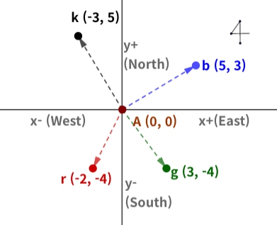
What does the Fig. 1.1 represent?
1) The x-axis and y-axis are based on East-West and South-North respectively.
2) It shows the position and distance of 4 points along each axis.
Fig. 1.1 Vector and coordinates.
The data in Fig. 1.1 could give a variety of meanings besides the meaning of directions. Whatever the interpretation, we can extract the two above.
The size and direction of each point can be calculated based on point A. For example, for point b, it is located at (5, 3) and the straight line distance from A is 4. This linear distance can be calculated using the famous Pythagorean theorem of a right triangle.
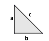
The length of each side of a right triangle is calculated by the Pythagorean Theorem shown below.
c = a +b
c=(a +b ) 1/2
In Fig. 1.1, the position of b is 5 on the x-axis and 3 on the y-axis, so it can be regarded as a right triangle with a base(b) of 5 and a height(a) of 3. That is, the straight line distance between the origin(A) and b is as follows.
In [1]: ab=(5**2+3**2)**0.5 # (52+32)
...: round(ab,2)
Out[1]: 5.83
Each point is calculated based on the origin(A) as above.
At point b, the length of the base is (5-0) and the height is (3-0). Therefore, formulating this relationship gives the following:
In [1]: import numpy as np
...: point=np.array([[5,3],
...: [3,-4],
...: [-2,-4],
...: [-3,5]])
...: print(point)
[[ 5 3]
[ 3 -4]
[-2 -4]
[-3 5]]
In [2]: import pandas as pd
...: d=[(point[I,0]**2+point[I,1]**2)**0.5
...: for I in range(4)]
...: re=np.c_[point, d]
...: re1=pd.DataFrame(re)
...: re1.columns=['x','y','distance']
...: re1.index=['b','g','r','k']
...: print(re1)
x y distance
b 5.0 3.0 5.830952
g 3.0 -4.0 5.000000
r -2.0 -4.0 4.472136
k -3.0 5.0 5.830952
Distance = [(x -x ) -(y -y ) ] 1/2 (Eq. 1.1)
x , y : start point
x , y : end point
As shown in Eq. 1.1, the coordinates of each point contain the direction and distance from the reference point and are called vectors. On the other hand, the size of each point, such as the distance, is called a scalar. It can be defined as:
Vector : values with magnitude and direction
Scalar : value with size only
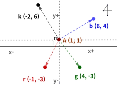
In Fig. 1.1, all coordinates are based on the origin(0, 0). However, if these default coordinates are not the origin, you can think that the coordinates themselves are shifted. For example, when A is moved to (1,1), it is changed as in Fig. 1.2.
Fig. 1.2 Shift of basic coordinates.
In the case of Fig. 1.2, the reference point A in Fig. 1.1 is moved from (0,0) to (1,1). This means that the reference axis is increased by 1 in the x and y directions, and all positions of each point are increased by the same amount. Therefore, the change of the basic axis induces the change of all other points, so the distance of each point will not change.
1.1.2 Dimension and axis
In Python, vectors and matrices that are a combination of multiple vectors can be represented using numpy's array(array object) . In particular, numpy's array objects are used not only for vectors and matrices, but also for the basic data types of most datasets to represent tables. For example, it is used as a basic type of sympy matrix objects used for vector or matrix operations, and pandas Series and DataFrame structures, which are important libraries for data analysis.
Numpy array objects can be created by the function. Each value of the array object created by this function has an index. This index indicates the position of the value within the object.
The argument of this function should be given in the form of a list, which is an ordered data type. One list represents one row .
In [1]: a=np.array([1,2]) #row vector
...: print(a)
[1 2]
In [2]: a1=np.array([[1],[2]]) #column vector
...: print(a1)
[[1]
[2]]
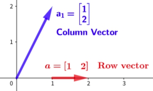
In the code above, object a consists of one row and is called a row vector . In the case of object a , it is an object composed of elements such as a, but it is called a column vector because it is in the form of one column.
Both vectors contain the same elements, but geometrically they have different meanings.
Fig. 1.3 Row vector and column vector.
As in Fig. 1.3, objects a and a both represent a line, but for a , they appear on one axis, but for a , on a plane formed by two axes, x and y. Therefore, a can be represented in one dimension, but a can only be displayed in two dimensions.


