Also by M.L. Humphrey
Listing of all books by M.L. Humphrey
Easy Excel Essentials 2019
Excel 2019 PivotTables
Excel 2019 Charts
Excel 2019 Conditional Formatting
Excel 2019 IF Functions
Excel Essentials 2019
Excel 2019 Beginner
Excel 2019 Intermediate
Excel 2019 Formulas & Functions
Access Essentials
Access for Beginners
Intermediate Access
Excel 2019 PivotTables
Easy Excel Essentials 2019 - Book
M.L. Humphrey
Contents
Introduction
PivotTables
Conclusion
Appendix A: Basic Terminology
About the Author
Copyright
Introduction
The Easy Excel Essentials 2019 series of titles are for intermediate-level users who want to focus on one specific topic such as PivotTables, Charts, Conditional Formatting, or the IF Functions.
The content of each title is extracted from either Excel 2019 Intermediate or Excel 2019 Formulas & Functions which cover intermediate-level Excel topics in more detail.
These books are written using Excel 2019 and assuming that a user is working in that program. If you are using an older version of Excel, the Easy Excel Essentials series may be a better choice since it was written using Excel 2013 and for a more general audience of Excel users.
With that introduction, lets dive in on how to use PivotTables.
PivotTables
Before we get started, for the record I passionately hate how they write PivotTable as one word with capital letters in the middle. But thats how they do it, so thats how well try to do it. (I may slip up once or twice, but Ill try to catch myself. While were on the subject I also passionately hate how their labels and menu options in their dialogue boxes dont use title case and so youll often see that I do.)
Alright then. Now that thats out of my system.
If you learn one intermediate-level Excel concept let it be PivotTables. I literally chose to write the first two books in the original Excel Essentials series for Beginners and Intermediate in order to teach writers how to use Excel well enough for them to use PivotTables.
Thats how useful these things are: I was willing to write thousands of words about the basics of Excel just to get people to the point where we are right now where I could teach them how to use PivotTables.
What They Do
So what are PivotTables? What do they do? Why are they so special?
A PivotTable takes rows and rows of data and lets you create a nice little summary table of that data based upon your chosen parameters.
Let me give you an example of how this can be useful.
Lets say you sell widgets, whatsits, and whatchamacallits. And every time you sell one of those items your distributor (the place you sell through) creates a line of data in an Excel worksheet that has the state where the sale occurred, the retail price, and the net amount due to you for that transaction, and you want to know what youve earned in each state so you can target advertising.
You could filter your data to see this or use subtotals even, but a far better option is to create a PivotTable of your data.
Lets do that. But first we need to cover some basic data principles.
Basic Data Principles
The data you use to build your table needs to be in the right format.
There should be one row at the top of your data table that contains the labels for each column. (I sometimes call this the header row.)
Everything needs to be in that one row. You cannot have multiple rows of column labels. So if youre going to have Year and Month, you cant put Year on Row A and then months on Row B, they need to be combined.
One header row.
Directly below the header row you put your data with one row per entry and nothing else in the midst of that data such as subtotals or grand totals.
Ideally your header row starts in Cell A1 followed by your data starting in Cell B1 and there is nothing else in the worksheet. But you can have data that starts elsewhere as long as once it starts its header row followed by rows of data and nothing else.
The mistake a lot of people make is that theyll list information in one row and then below that row list a subset of information.
So maybe Row is the customer information and then below that in Rows 6-10 is the transaction information and then Row is a row for total values for that customer.
Dont do that. That is a report. That is something that is meant to be final and no longer subject to analysis. If youre still going to work with your data, leave it as raw and untouched as you can. Once you put in subtotals or break your data up into multiple lines, you cant sort it, filter it, use PivotTables, or create charts from it.
So dont do that. At least not in your source worksheet.
(As discussed more in Data Principles for you should always have one place where you store your raw data.. You can then use that information to create your summary reports and analysis, or even fix the data. But always have that one document that is just the information and that is not changed or touched or messed with in any way so that you can go back to it if you make a mistake.)
(This helps especially if you sort your data wrong because that can pretty much break your data and you cant fix it. Keeping your source data pure lets you go back and start over.)
Also be sure to not have any blank rows or columns in your data set and to have only one type of data (date, currency, text) per column.
Blank rows arent a deal-breaker, but Excel will treat them as valid sources of data so youll end up with blank entries in your PivotTables.
Blank columns will generate an error message when you try to create the PivotTable because there is no valid field name for Excel to use for that column(s).
Various types of data in one column makes it almost impossible or at least very challenging to create any sort of analysis based on that data.
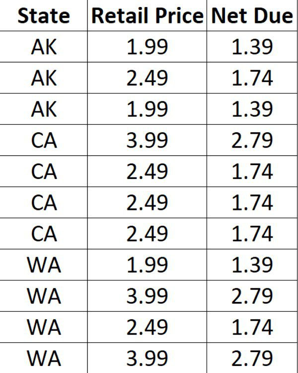
Okay. If you want to learn more about setting up your data in the best possibly way, check out Data Principles for but were going to move on now and create a PivotTable with one parameter using the following data table that shows state, retail price, and net due.
Building a Pivot Table
The PivotTable we want to build is going to calculate Net Due for each possible state. The initial steps for building a PivotTable are the same no matter how complex youre going to make that table.
First, highlight your data.
If its the entire worksheet, you can just Select All by clicking in the top left corner or using Ctrl + A. If the data starts lower down in the worksheet or you just want to use a subset of your data then highlight the rows you want.
Be sure to highlight the header row as well as the data rows. This does not work if you do not have a header row. Furthermore, the header row must be next to the rows of data that you want to analyze.
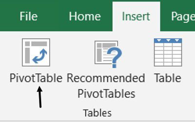
Once you have your data selected, go to the Insert tab and in the Tables section on the left side choose PivotTable.


