Sheikh - Microsoft Excel Advanced Functions and Formulas

Excel Advanced Functions and FormulasAhmed Sheikh,M.Sc. (USA)TABLE OF CONTENTSUnit 1: Building complex formulasIn this unit, you will learn how to: Work with nesting functions Compare results between using a formula with nested IF vs. a VLOOKUP Use the VLOOKUP with the COLUMN function Source table structure information using CHOOSE function Use INDEX and MATCH to search for information Formulas and worksheet functions are essential to manipulating data and obtaining useful information from your Excel workbooks. This section includes formulas containing functions such as IF, AND, OR, NOT, CHOOSE, VLOOKUP, COLUMN, INDEX and MATCH and to make it more challenging the examples that will be used include combinations of these functions in the same formula. Using nested IF statements In Excel the 'IF' function is commonly used as it provides solutions for many complex and varying situations in Excel. Let's begin with a formula containing multiple IF functions, also known as a nested IF formula.

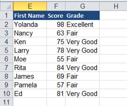
It is necessary to understand the syntax of this function which is as follows: IF(Logical Test, Value if True, IF(Logical Test, Value if True, IF(Logical Test, Value if True, Value if False))) In the above example there are three logical tests which produce a value if true followed by a final result if none of the IF statements are true. The following is an example showing grading comments based on score results. =IF(F2>=90,"Excellent", IF(F2>=70,"Very Good", IF(F2>=50,"Fair","Poor"))) To examine the formulas in more detail take a look at the following screenshot showing the breakdown of the nested IF formula which produces the required results. Creating compound logical tests using AND, OR, NOT functions with IFstatements Using an IF function by itself in a formula works when there are no special conditions to be added. When the results are based on conditions then you have to nest the IF function with either the AND function or with the OR function. The AND function can hold up to 255 logical tests, however, to arrive at a result which is TRUE all the logical tests must be true.

This makes the AND function quite restrictive in its use. On the other hand the OR function, which can also hold up to 255 logical tests, requires that only one of its logical tests be true in order to arrive at a result which is TRUE. In the following screenshot the Excel spreadsheet represents sales data and we will be using the IF function together with AND, NOT and VLOOKUP to work out bonus calculations. To pay a 2% bonus for sales greater than 20000 we would use a formula with a simple IF function that would be as follows: =IF(F2>20000,0.02*F2,0) But what if we decided that the bonus would only be paid if the GP% is greater than 50% in addition to the first condition that sales must be greater than 20000? We could then use two IF functions one to deal with the first logical test and then the second to deal with the new logical test. The formula to produce the desired result would look like this: =IF(F2>20000,IF(I2>0.5,0.02*F2,0),0) The exact same result can be achieved by using the following formula which incorporates both the IF and the AND functions. =F2*0.02*(F2>20000)*(I2>0.5) This formula starts out by calculating a 2% bonus for everyone: F2*0.02. =F2*0.02*(F2>20000)*(I2>0.5) This formula starts out by calculating a 2% bonus for everyone: F2*0.02.

But then the formula continues with two additional terms both of which must be in parentheses. Excel treats (F2>20000) as a logical test and will evaluate that expression to either TRUE or FALSE and will do the same with (I2>0.5). So, for row 2 the intermediate step will appear as follows: =22810*0.02*TRUE*FALSE When Excel has to use TRUE or FALSE in a calculation, the TRUE is treated as a one. The FALSE is treated as a zero. Since any number times zero is zero, the logical tests at the end of the formula will wipe out the bonus if any one of the conditions is not true. The final step of the calculation will be as follows: =22810*0.02*1*0 which will equal zero.

In row 7, the calculation will be =21730*0.02*TRUE*TRUE which becomes =21730*0.02*1*1 giving a result of 434.60. 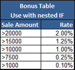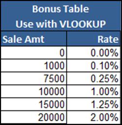Comparing a nested IF formula with VLOOKUP What if your bonus rates were based on a sliding scale? You could use a nested IF formula which would evaluate each level starting with the largest category first. The bonus table would look as follows: The formula would be: =IF(F3>20000,$N$6,IF(F3>15000,$N$7,IF(F3>10000,$N$8,IF(F3>7500,$N$9,IF(F3> 1000,$N$10,0)))))*F3 To produce the same result with a VLOOKUP function the bonus table must be modified to the following: The formula would be as follows: =VLOOKUP(F3,CommTable,2)*F3 where the range name 'CommTable' refers to M16:N21. Using the NOT function The NOT function can also be used in formulas to reverse the TRUE or FALSE result. We will use the NOT function in a formula which uses the IF function, together with the AND function. The formula will be as follows: =IF(NOT(AND(F3>20000,J3=$O$6)),F3*0.02,0) Cell F3 contains the sales value and cell O6 contains the rep's name.

Normally, the AND function will produce a result if both logical tests are true, but with the NOT function in the picture, the results are reversed. 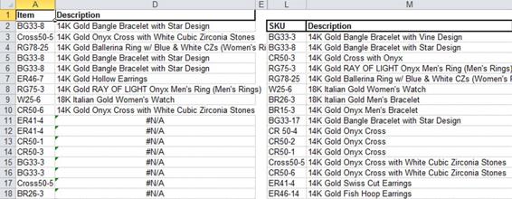Nesting VLOOKUP functions A common practice in Excel is to download data from other data sources. This often presents a problem when the data contains leading, trailing or extra unwanted spaces. So, when using a VLOOKUP function a lookup column containing trailing/extra spaces can cause #N/A errors to occur. The way around this is to add the TRIM function to the formula which immediately eliminates the spaces so that the lookup column data will match with the table array data. Should the table array have any unwanted spaces, this can be dealt with in a similar fashion but with an added twist to the formula.

The first result using TRIM before the table array will produce a #VALUE! error. This can be resolved by entering the formula by holding down the CTRL + SHIFT buttons and then pressing the enter key. This is known as an array formula and will be covered in more detail in a later unit called Array Functions. =VLOOKUP(TRIM(A2),Products,2,FALSE) =VLOOKUP(A11,Products,2,FALSE) Using VLOOKUP with the COLUMN function The formula =VLOOKUP($A4,$H$4:$L$227,2,FALSE) is in cell B4 in the above example. When this is copied across the row number will not change and therefore the results are all the same. This can be overcome by numbering B1 to 2, C1 to 3, D1 to 4 and E1 to 5 then modifying the formula to the following =VLOOKUP($A4,$H$4:$L$227,B$1,FALSE).