Galina Filipuk - Multi-variable Calculus: Vol 2
Here you can read online Galina Filipuk - Multi-variable Calculus: Vol 2 full text of the book (entire story) in english for free. Download pdf and epub, get meaning, cover and reviews about this ebook. year: 2020, publisher: De Gruyter, genre: Children. Description of the work, (preface) as well as reviews are available. Best literature library LitArk.com created for fans of good reading and offers a wide selection of genres:
Romance novel
Science fiction
Adventure
Detective
Science
History
Home and family
Prose
Art
Politics
Computer
Non-fiction
Religion
Business
Children
Humor
Choose a favorite category and find really read worthwhile books. Enjoy immersion in the world of imagination, feel the emotions of the characters or learn something new for yourself, make an fascinating discovery.

- Book:Multi-variable Calculus: Vol 2
- Author:
- Publisher:De Gruyter
- Genre:
- Year:2020
- Rating:4 / 5
- Favourites:Add to favourites
- Your mark:
Multi-variable Calculus: Vol 2: summary, description and annotation
We offer to read an annotation, description, summary or preface (depends on what the author of the book "Multi-variable Calculus: Vol 2" wrote himself). If you haven't found the necessary information about the book — write in the comments, we will try to find it.
Galina Filipuk: author's other books
Who wrote Multi-variable Calculus: Vol 2? Find out the surname, the name of the author of the book and a list of all author's works by series.


![Chris Monahan [Chris Monahan] - Calculus II](/uploads/posts/book/119088/thumbs/chris-monahan-chris-monahan-calculus-ii.jpg)
Multi-variable Calculus: Vol 2 — read online for free the complete book (whole text) full work
Below is the text of the book, divided by pages. System saving the place of the last page read, allows you to conveniently read the book "Multi-variable Calculus: Vol 2" online for free, without having to search again every time where you left off. Put a bookmark, and you can go to the page where you finished reading at any time.
Font size:
Interval:
Bookmark:
De Gruyter Textbook
ISBN 9783110660388
e-ISBN (PDF) 9783110660395
e-ISBN (EPUB) 9783110660418
Bibliographic information published by the Deutsche Nationalbibliothek
The Deutsche Nationalbibliothek lists this publication in the Deutsche Nationalbibliografie; detailed bibliographic data are available on the Internet at http://dnb.dnb.de.
2021 Walter de Gruyter GmbH, Berlin/Boston
Mathematics Subject Classification 2010: 97I20, 97I60, 53A04, 53A05, 97N80,
In this book we shall deal with mappings from a subset URn to Rm for arbitrary positive integers m and n, where at least one of them is greater than one. Such mappings f are given as collections of m functions (f1,f2,,fm) , where fi:UR is a function of n variables. Usually, for m=1 , they are called functions and for m>1 mappings (maps, vector-valued functions).
In this chapter we first deal with Rn and introduce the notions of metric, norm, inner product, and discuss relations between them. Then we define the notions of limits, topology, and continuous mappings. We show how to visualize mappings in Mathematica and study their continuity. As an application we illustrate how continuous mappings can be used to analyze the topological properties of sets.
Recall that a metric space is a set X together with a map d:XXR0 with the following properties [, p.650]:
d(x,y)=0 if and only if x=y ;
d(x,y)=d(y,x) ;
d(x,z)d(x,y)+d(y,z) (triangle inequality).
Mathematica has many built-in functions containing the word distance as one can check by typing
| In[]:= | ?*Distance |
For instance, EuclideanDistance , HammingDistance , GraphDistance , TravelDistance , and many others. However, not all of them refer to a distance in our sense. The most general, applicable to any set X, is the function BinaryDistance :
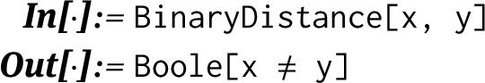 In this metric the distance between any element and itself is 0, and the distance between any unequal elements is 1. It is easy to verify the triangle inequality by hand. If we try to use Mathematica for this purpose, we obtain a somewhat strange result:
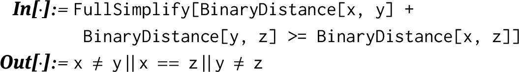 Of course, this relationship should evaluate to True . However, Mathematica cannot simplify such expressions unless it knows that the symbols represent real (or complex) numbers:
| In[]:= | FullSimplify[%, Assumptions -> Element[_, Reals]] |
| Out[]:= | True |
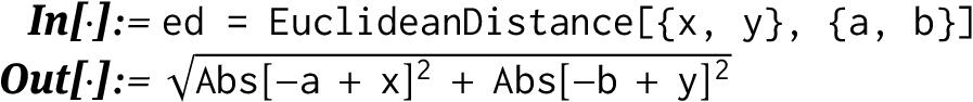
The most important distance for us will be the EuclideanDistance . It is normally defined on the Cartesian product Rn , but since Mathematica by default works over the complex numbers, it computes the distance in Cn :
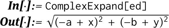
 One way to deal with this is to apply the function ComplexExpand , which by default assumes that all parameters are real:
 We can also use ComplexExpand to see that the distance on the set Cn is just the Euclidean distance on R2n :
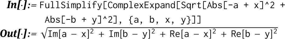 Note that ComplexExpand treats all variables as real unless they are listed in the second argument.
Other useful distances on Rn are ManhattanDistance and ChessboardDistance :
| In[]:= | ManhattanDistance[{x, y, z}, {a, b, c}] |
| Out[]:= | Abs[-a + x] + Abs[-b + y] + Abs[-c + z] |
| In[]:= | ChessboardDistance[{x, y, z}, {a, b, c}] |
| Out[]:= | Max[Abs[-a + x], Abs[-b + y], Abs[-c + z]] |
As can be seen from the above, the ManhattanDistance between two points is the sum of the distances between their projections on the coordinate axes, while the ChessboardDistance is the maximum of these distances. It is easy to show that both satisfy the triangle inequality.
A very important consequence of having a metric on a set X is that it defines a topology on X. In order to define a topology on X, we need the notion of an open set, and to define open sets, we need the notion of an open ball. The open ball with center at x0 of radius r>0 is the set B(x0,r)={xX|d(x,x0) . A subset YX is called a neighborhood of yY if there is an r>0 such that B(y,r)Y . A subset UX is said to be open if it is a neighborhood of its every point. Closed sets are the complements of open sets. Clearly, the empty set and the whole space X are both open and closed sets.
To understand open sets with respect to a metric, we need to understand the open balls. The following function draws a ball of a given radius for a given metric:
| In[]:= | ball[metric_, r_] := RegionPlot[metric[{x, y}, {0, 0}] |
| < r, {x, -2*r, 2*r}, {y, -2*r, 2*r}] |
Note that since RegionPlot never draws objects of dimension less than two, it will not correctly represent ball[BinaryDistance, 1] , which is a point (actually the picture is empty). Let us consider the balls in the following metrics:
| In[]:= | {ball[EuclideanDistance, 1], ball[ManhattanDistance, 1], |
| ball[ChessboardDistance, 1]} |
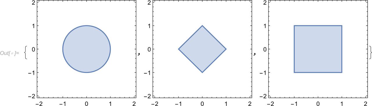
We can now see that although the open balls in these metrics have different shapes, a ball in each metric contains and is contained in a ball of any other metric:
| In[]:= | Show[(ball[#1[[1]], #1[[2]]] & ) /@ |
| {{EuclideanDistance, 1}, {ManhattanDistance, 1/2}, | |
| {ChessboardDistance, 1/4}, {EuclideanDistance, 1/8}}] |
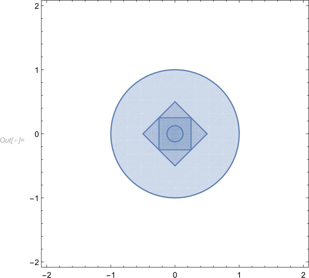
This implies that any open set with respect to any of these metrics is also open with respect to any other of these three metrics.
We say that two metrics d1 and d2 on X are equivalent if there exist constants c1>0 and c2>0 such that c1d1(x,y)d2(x,y)c2d1(x,y) for all x,yX . It is easy to see that all the metrics above are equivalent. Clearly, the binary metric is not equivalent to them.
Font size:
Interval:
Bookmark:
Similar books «Multi-variable Calculus: Vol 2»
Look at similar books to Multi-variable Calculus: Vol 2. We have selected literature similar in name and meaning in the hope of providing readers with more options to find new, interesting, not yet read works.
Discussion, reviews of the book Multi-variable Calculus: Vol 2 and just readers' own opinions. Leave your comments, write what you think about the work, its meaning or the main characters. Specify what exactly you liked and what you didn't like, and why you think so.