Since survival time is usually a continuous number, why not use ordinary regression analyses where survival time is the dependent variable (outcome)? Because survival time cannot be negative, linear regression models would be skewed.
Moreover, because the dependent variable in survival analysis has two aspects: time to event and status, ordinary regression models cannot answer two important questions: Q1) whats the probability of surviving past a point in time (survival function)? Q2) whats the failure rate to a certain point in time (also known as hazard function)? E.g.; how many will die by the age of 75? How many years will the machine work properly before we need to buy a new one?
Parametric, Non-parametric and Semi-parametric Survival Analysis
The table below summarizes the differences between the three approaches. Detailed examples are presented in the following chapters.
| Parametric | Non-parametric | Semi-parametric |
| Assume knowledge of the statistical distribution of survival times | Make no assumptions on the distribution of survival times like Kaplan Meier estimator | Has parametric and non-parametric components like the Cox regression model |
Example 2: Exploratory Analyses
The ovarian cancer data comes with the survival package in R. The following few commands explore the data. install.packages("survival",repos="http://cran.r-project.org") #install survival library library(survival) # load survival library > data(ovarian) > dim(ovarian) # Ovarian data has 26 rows and 6 columns [1] 26 6 > help(ovarian) starting httpd help server ... 1st Qu. 1st Qu.
Median Mean 3rd Qu. Max. 59.0 368.0 476.0 599.5 794.8 1227.0 > summary(age) # subjects age Min. 1st Qu. Median Mean 3rd Qu. 38.89 50.17 56.85 56.17 62.38 74.50 > cor(futime, age) # pair-wise correlation [1] -0.6483612 > psymbol<-fustat+1 > table(psymbol) # 2 = censored psymbol 1 2 14 12 > plot(age, futime) 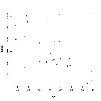
plot(age, futime, pch=(psymbol)) 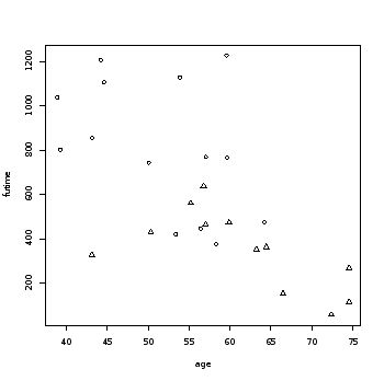 > detach(ovarian)# so the variables do not overlap Interpretation: This dataset had 26 subjects (patients), and 12 censored observations (fustat). 38.89 50.17 56.85 56.17 62.38 74.50 > cor(futime, age) # pair-wise correlation [1] -0.6483612 > psymbol<-fustat+1 > table(psymbol) # 2 = censored psymbol 1 2 14 12 > plot(age, futime)
plot(age, futime, pch=(psymbol))  > detach(ovarian)# so the variables do not overlap Interpretation: This dataset had 26 subjects (patients), and 12 censored observations (fustat).
Survival time ranged from 59 to 1227 weeks, with an average of 599.8 weeks. The patients ages averaged at 56 years and ranged from 38.9 to 74.5 years. The first plot contrasts survival time against age regardless of censored status. Notice that as age increases survival time decreases. This is also manifested in the negative strong pairwise correlation between the two (-0.65) . The second plot differentiates the subjects with censored status (triangle = censored).
Censored ones are presented with triangles. They show relatively lower survival time.
Chapter 2: Parametric Survival Analysis
This approach assumes that survival time data follows a certain distribution like exponential, Weibull, lognormal, log logistic, or generalized gamma. It rarely, if ever follows a normal distribution. Not all R functions support all of these distributions, so you will need to read the documentation of the function in order to find out which distribution it supports.
Example 3: Fitting a Parametric Model
This comprehensive example explores the larynx cancer data which is available from the KMsurv package. >install.packages("KMsurv",repos="http://cran.r-project.org") > library(KMsurv) Warning message: package KMsurv was built under R version 3.1.3 > data(larynx) help(larynx) Description The larynx data frame has 90 rows and 5 columns. >install.packages("KMsurv",repos="http://cran.r-project.org") > library(KMsurv) Warning message: package KMsurv was built under R version 3.1.3 > data(larynx) help(larynx) Description The larynx data frame has 90 rows and 5 columns.










 > detach(ovarian)# so the variables do not overlap Interpretation: This dataset had 26 subjects (patients), and 12 censored observations (fustat). 38.89 50.17 56.85 56.17 62.38 74.50 > cor(futime, age) # pair-wise correlation [1] -0.6483612 > psymbol<-fustat+1 > table(psymbol) # 2 = censored psymbol 1 2 14 12 > plot(age, futime)