Bob Umlas - Cool Excel Sh*t

Cool Excel Sh*t 2021 by Bob Umlas and Holy Macro! Books All rights reserved. No part of this book may be reproduced or transmitted in any form or by any means, electronic or mechanical, including photocopying, recording, or by any information or storage retrieval system without written permission from the publisher. All terms known in this book to be trademarked have been appropriately capitalized. Trademarks are the property of their respective owners and are not affiliated with Holy Macro! Books. Every effort has been made to make this book as complete and accurate as possible, but not warranty or fitness is implied. The information is provide on an as is basis.

The author and the publisher shall have neither liability nor responsibility to any person or entity with respect to any loss or damages arising from the information contained in this book. Printed in the USA by Hess Print Solutions First Printing: April 2022 (e-book April 2021) Author: Bob Umlas Cover Design: Shannon Travise Publisher: Bill Jelen Index: Nellie Jay Tech Editor: Bill Jelen Published by Holy Macro! Books, PO Box 541731, Merritt Island FL 32954 Distributed by Independent Publishers Group, Chicago IL ISBN 978-1-615470-073-0 (print) 978-1-615470-159-1 (digital) Library of Congress Control Number: 2021TBD Table of Contents Other books by Bob Umlas: This isnt Excel, its Magic (2005) This isnt Excel, its Magic 2nd Edition (2007) Excel Outside the Box (2012) More Excel Outside the Box (2015) Excel Preschool (2019) Foreword I actually learned Microsoft Excel on the Macintosh in 1986 or so, using version 0.99! When the real version (1.00?) shipped, I read the manual (yes, Excel came with manuals then) from cover to cover. Six times. Especially in order to learn Data Tables. I just didnt get it. (Okay, so Im a geek.

Actually, I once heard that youre a geek if you double-click the TV remote)! Around 1993 I received the nickname Excel Trickster from one Will Tompkins, a real Excel Guru. I got that because during a seminar he was hosting in Washington, I believe, for what he called the Excel SWAT team, he was showing his then famous Tompkins methodology a macro structure using Excel 4 style macros (before VBA existed in Excel) which was quite sophisticated. He showed a line of code which used a range name, a label, and he wanted to show us the code at that label. So, he used F5(Goto), and we saw literally many hundreds of defined names which he had to laboriously scroll through to get to the one he was looking for. After he had done this about 4-5 times, I raised my hand and said, You know, you can get to that label directly. Just press Ctrl/[.

He tried it and was flabbergasted! So, he tried it again. Then he remarked that I just saved him about 2 hours every day scrolling through his defined names! When I also told him you could return to the location you were just at by using Ctrl/], he called me the Excel Trickster, and that nickname has stuck with me ever since. So, thank you, Will. Ive been an Excel MVP for 25 years 1993-2018, and I currently lead an online Master Class in Excel which is 12 3-hour sessions and a VBA class which is 2 3-hour sessions. I have presented at various global events (EIEFreshTalk and GlobalExcelSummit) with 1750 and 9400+ participants, respectively! Acknowledgments Id like to thank my wife, Judy, for her continued support of my pursuing my Excel studies, former and current Excel MVPs for their continued eye-opening ideas upon which I have built some of these ideas. Several ideas in this book were first discussed in the 2007 book, This Isnt Excel, Its Magic, published by IIL Publishing in New York.

That book features 111 Excel tips and is still available from the publisher . FORMULAS An amazing formula to SUMIF the visible rows This isnt so much a tip/trick (its a bit advanced), but worth visiting! Lets look at a worksheet containing the source data: 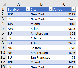And lets say this goes down to row 123. I inserted a slicer for this data: 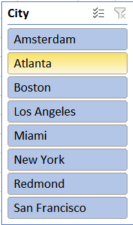then I cut this slicer and pasted it to another sheet: 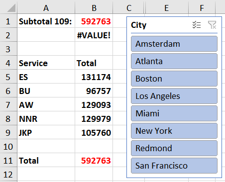Its fairly straightforward to get the right formula in cell B1 to add up all the values from the source sheet, depending on the choices in the slicer: =SUBTOTAL(109,Supporting Data!C:C) This is because the choices in the slicer will hide/show the appropriate rows and the SUBTOTAL(109, will summarize the unhidden rows. But how can you further break it down by service so the numbers in B5:B9 can be determined? The #VALUE! Error in B2 is a first attempt. We need to pretty much use the same SUBTOTAL formula as in B1, but perhaps pass this to a SUMPRODUCT formula: =SUMPRODUCT(SUBTOTAL(109,Supporting Data!C2:C123),N(Supporting Data!$A$2:$A$123=A5)) This seems like it should work but it gives that #VALUE! error. Why? Its because the first part (the SUBTOTAL) gives just one value, and the 2nd part gives an array of values: It becomes =SUMPRODUCT( 592763 ,N(Supporting Data!$A$2:$A$123=A5)) which becomes =SUMPRODUCT( 592763 ,{0;1;0;0;0;1;0;0;0;0;0;1;0; 0;0;0;0;1;1;0;1;1;0;0;0;0;0;0;0;0;0;0;1;0;0;0;1;0;0;0;1;0;0;1;0;0;0;0;0;1;0;0;0;0;0;1;0;1;0;1;0;0;0;0;0;0;0;0;1;0;0;0;0;0;1;0;0;0;0;0;0;1;0;0;0;1;0;0;0;0;0;0;0;0;0;0;0;0;0;0;1;0;0;0;0;0;0;0;0;0;0;1;1;0;0;1;0;1;0;0;1;0}) which simply doesnt balance.

There needs to be the same number of values in each section. So how do we make this happen? Lets look at the solution and see how it works: =SUMPRODUCT(SUBTOTAL(109,OFFSET(Supporting Data!$C$1,
SEQUENCE(122),0)),N(Supporting Data!$A$2:$A$123=A5)) does the job. Lets break this down. The magic is really in the OFFSET formula: This expands to the following: Notice that we now are going to have the same number of values in each argument to the SUMPRODUCT function. The above expands to: And the result is what were looking for. SEQUENCE(122) generates values 1,2,3,122 and the offset from C1 for 1,2,3122 is C2, C3, C4,,C123 where C123 is the last cell in the source data.

This could also have been OFFSET(Supporting Data!$C$1,ROW($1:$122),0) using ROW instead of SEQUENCE. This responds to the slicer settings (the formula in B5 is shown via a
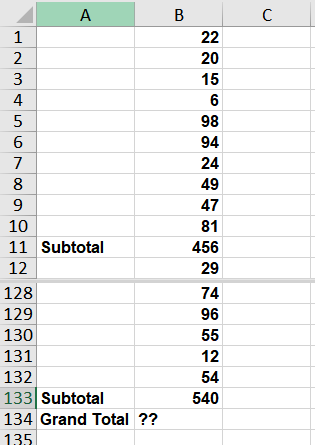
FORMULATEXT in H5): 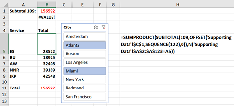Putting in a Grand Total of data already subtotaled Suppose you have a worksheet which looks like this (note that the screen is split and rows 13:127 are not shown):