LitArk » Books » Computer

Sibley Kelvin - 2021 Microsoft Formulas and Functions: A Simplified Guide With Examples on how to take advantage of built-in Excel Formulas and Functions

Here you can read online Sibley Kelvin - 2021 Microsoft Formulas and Functions: A Simplified Guide With Examples on how to take advantage of built-in Excel Formulas and Functions full text of the book (entire story) in english for free. Download pdf and epub, get meaning, cover and reviews about this ebook. year: 2021, genre: Computer. Description of the work, (preface) as well as reviews are available. Best literature library LitArk.com created for fans of good reading and offers a wide selection of genres:

Romance novel Science fiction Adventure Detective Science History Home and family Prose Art Politics Computer Non-fiction Religion Business Children Humor

Choose a favorite category and find really read worthwhile books. Enjoy immersion in the world of imagination, feel the emotions of the characters or learn something new for yourself, make an fascinating discovery.

Book:
2021 Microsoft Formulas and Functions: A Simplified Guide With Examples on how to take advantage of built-in Excel Formulas and Functions
Author:
Sibley Kelvin
Genre:
Books / Computer
Year:
2021
Rating:
4 / 5
Favourites:
Add to favourites
Your mark:
- 80
- 1
- 2
- 3
- 4
- 5

Description
Author's other books
Similar books

2021 Microsoft Formulas and Functions: A Simplified Guide With Examples on how to take advantage of built-in Excel Formulas and Functions: summary, description and annotation

We offer to read an annotation, description, summary or preface (depends on what the author of the book "2021 Microsoft Formulas and Functions: A Simplified Guide With Examples on how to take advantage of built-in Excel Formulas and Functions" wrote himself). If you haven't found the necessary information about the book — write in the comments, we will try to find it.

You can master the use of over 101 Microsoft Excel Formulas and Functions if you make the decision to purchase this book.This guide is what should be called; a one-fit approach to understanding the basis of Excel formulas. This guide is useful especially for business owners, workers, and financial analysts who want to up their game with Excel, and use Excel formulas like a professional. The guide has been designed, equally, to suit the taste of individuals; who are not business inclined and who only want to learn about useful formulas in Excel. The book is replete with images and annotations to drive home the essence of each formula.A snippet of what you will get in this book include:How to delete a formula but keep the result of the formula (for Windows users)Avoiding broken formula in ExcelEXCEL FORMULA COMMONLY USED IN BUSINESS ANALYTICSMANIPULATING TEXTS WITH FORMULAHow to use the TRIM Function in ExcelHow to use the FVSCHEDULE Function in ExcelHow to employ the ACCRINT Function in ExcelHow to use the CUMIPMT Function in ExcelHow to use the FV Function in ExcelHow to use the IPMT Function in ExcelHow to use the NPER Function in ExcelHow to use the PDURATION Function in ExcelHow to use VLOOKUP in ExcelHow to use the CELL function in ExcelHow to use the Excel ISBLANK FunctionHow to use the ISERROR Excel FunctionHow to deploy the ISEVEN Function in ExcelHow to create conditional formattingHow to deploy the ISTEXT Function in ExcelHow to use the TYPE Function in ExcelHow to employ the AND Function in ExcelHow to use the NOT Function in ExcelCalculating Gross Profit Margin and Gross Profit MarginCalculating the EBIT and EBITDACalculating Cost of Goods SoldCalculating Return on AssetsCalculating Break EvenCalculating Customer ChurnAnd Lots moreScroll up and click the BUY NOW Button to get started

Sibley Kelvin: author's other books

Who wrote 2021 Microsoft Formulas and Functions: A Simplified Guide With Examples on how to take advantage of built-in Excel Formulas and Functions? Find out the surname, the name of the author of the book and a list of all author's works by series.

2021 Microsoft Formulas and Functions: A Simplified Guide With Examples on how to take advantage of built-in Excel Formulas and Functions — read online for free the complete book (whole text) full work

Below is the text of the book, divided by pages. System saving the place of the last page read, allows you to conveniently read the book "2021 Microsoft Formulas and Functions: A Simplified Guide With Examples on how to take advantage of built-in Excel Formulas and Functions" online for free, without having to search again every time where you left off. Put a bookmark, and you can go to the page where you finished reading at any time.

Light

Font size:

↓

↑

Reset

Interval:

↓

↑

Bookmark:

Make

2021 Microsoft

Excel Formulas and Functions

A Simplified Guide with Examples on How to Take Advantage of Built-in Excel Formulas and Functions

Kelvin Sibley

ChurchGate Publishing House

USA | UK | Canada

Churchgate Publishing House 2021

All rights reserved. No part of this publication may be reproduced, stored in a retrieval system or transmitted in any form or by any means, electronic, mechanical, photocopying, recording, and scanning without permission in writing by the author.

While the advice and information in this book are believed to be true and accurate at the date of publication, neither the authors nor the editors nor the publisher can accept any legal responsibility for any errors or omissions that may be made. The publisher makes no warranty, express or implied, with respect to the material contained herein.

Printed on acid-free paper.

Printed in the United States of America

2021 by Kelvin Sibley

Table of Contents

CHAPTER ONE

BRIEF INTRODUCTION TO SOME EXCEL BASIC

Before we dabble into the main aspect of this guide which is the Excel tips, tricks and formulas let us examine some basic Excel stuff.

How does the formula in Excel look?

When you take a cursory look at the image above you will obviously observe - photo 1

When you take a cursory look at the image above, you will obviously observe some numbers ranging from 1 to 4. That is the basic Excel formula, and you might be interested in knowing what the numbers stand for;

- The number 1 represents Functions: The number (circled 1) is the pi function and its function is to always return the value of pi, which is always equal to 22/7, or 3.142

- References: The number A2 will normally return the exact value in the cell A2.

- Constants: The number (circled as 3) always stands for constant, which are numbers that are just inherently there in the formula.

- Operators: The caret ^ operator in the formula above will usually raise a certain number to a particular power and indicate its value.

Define and use names in Excel formula

Deploying names in your formula makes the formula look neater, explicable and very easy to maintain. You can define names for your constant, table, function or cell range. Once you adopt the act of using names in your Excel workbook, the names then become especially easier to update, audit and manage.

Naming a cell (For Windows users)

- Select a cell.

- Input a name in the Name box.

- Click Enter.

Define names from a selected range

- Select the range that you plan to name, including the column or row labels.

- Choose Formulas, and tap Create from Selection.

- From the dialog box of the Create Names from Selection , assign the location containing the labels by clicking on the Left column, Top row , Bottom row , or the Right column check box.

- Click OK .

Excel will assign names to the cells based on the labels in the designated range.

Managing names in your workbook with Name Manager

On the Ribbon, navigate to Formulas, click on Defined Names and select Name Manager . From there, you can create, delete, edit and locate all the names deployed in the workbook.

Naming a cell (For macOS users)

Pick a cell.
Fill in a name inside the Name Box.

Tap Enter.

Define names from a selected range

- Click on the range that you plan to name, including the row label or column.

- Click on Formulas, and click on Create from Selection.

- From the Create Names from Selection dialog box, assign the location containing the labels by tapping on the Left column, Top row , Bottom row , or the Right column check box.

- Select OK .

The Microsoft Excel will give names to the cells based on the labels in the designated range.

Use names in formulas

- Select a cell and enter your formula.

- Place the cursor of your computer at the exact place or point where you want the name to be used in the formula.

- Input the first letter of the name, and select the name from the list shown.

- Alternatively, select Formulas , click on Use in Formula and tap or select the name that you plan to use.

- Tap Enter.

Deleting or removing a formula in your Excel workbook

When you delete a particular formula, you should know that the result of that particular formula is also deleted automatically. To avoid this, you can instead just remove the formula instead of deleting it in its entirety. This way, the result of the formula is not deleted. However, if you still want to delete a formula, you can use the steps below;

- Select the cell or choose the range of cells that contain the said formula.

- Click on Delete.

How to delete a formula but keep the result of the formula (for Windows users)

To delete a formula while keeping the result of the formula, you will need to copy the formula and then paste the formula in the same cell using the Paste Values option. Follow the prompts below;

Select the cell or choose the range of cells that contains the said formula.
In the instance where the said formula is actually an array formula, then you will have to select all of the cells in the range of cells containing the array formula.
1. Click on a cell from the array formula.
2. From the Home tab, under the Editing group, click on Find & Select , and then click on Go To .
3. Click on Special .
4. Select Current array .
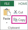
From the Home tab, in the Clipboard group, choose Copy .
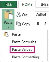
From the Home tab, in the Clipboard group, click on the arrow below Paste , and then select Paste Values .

Delete an array formula

If you plan to delete a certain array formula, you will need to make sure that all the cells in the cell range that contain the array formula are chosen. To do this;

Choose a cell from the array formula.
From the Home tab, under the Editing group, click on Find & Select , and then click on Go To .
Click on Special .
Select Current array .
Tap DELETE .

Delete a formula but keep the results (for web users)

Click on the cell or the range of cells where the formula is located.
Click on Home , and select Copy (or simply use the Ctrl + C shortcut).

Choose Home click on the arrow below Paste and choose Paste Values - photo 6

Choose Home , click on the arrow below Paste and choose Paste Values .

Avoiding broken formula in Excel When the Microsoft Excel is not able to - photo 7

Light

Font size:

↓

↑

Reset

Interval:

↓

↑

Bookmark:

Make

Similar books «2021 Microsoft Formulas and Functions: A Simplified Guide With Examples on how to take advantage of built-in Excel Formulas and Functions»

Look at similar books to 2021 Microsoft Formulas and Functions: A Simplified Guide With Examples on how to take advantage of built-in Excel Formulas and Functions. We have selected literature similar in name and meaning in the hope of providing readers with more options to find new, interesting, not yet read works.

Alan Murray

Advanced Excel Formulas: Unleashing Brilliance with Excel Formulas

Ahamed Mohideen Mubeen

Most Essential Excel Formulas and Functions for Any Career: VLOOKUP, Excel Formulas and Functions

Sheikh

Microsoft Excel Advanced Functions and Formulas

JORDAN

EXCEL 2021 FOR BEGINNERS: THE COMPLETE DUMMY TO EXPERT PRACTICAL GUIDE WITH EXAMPLES THAT TEACHES EVERYTHING YOU NEED TO KNOW ABOUT MICROSOFT EXCEL 2021 (FORMULAS, FUNCTIONS, VBA & MACROS INCLUSIVE)

Baddey

EXCEL 2020 EXPLAINED: A Well-Explained Guide to Master Microsoft Excel Functions and Formulas from Beginner to Expert Level

Bluttman

Microsoft Excel formulas & functions for dummies

Alexander Michael

Excel 2016 Formulas

Alexander Michael

101 Ready-to-Use Excel Formulas

Harjit Suman

Excel Formulas and Functions : the Complete Excel Guide for Beginners

Suman

Excel Formulas and Functions: The Step by Step Excel Guide on how to Create Powerful Formulas

John Michaloudis

101 Most Popular Excel Formulas

John Walkenbach

Excel 2013 Formulas

Reviews about «2021 Microsoft Formulas and Functions: A Simplified Guide With Examples on how to take advantage of built-in Excel Formulas and Functions»

Discussion, reviews of the book 2021 Microsoft Formulas and Functions: A Simplified Guide With Examples on how to take advantage of built-in Excel Formulas and Functions and just readers' own opinions. Leave your comments, write what you think about the work, its meaning or the main characters. Specify what exactly you liked and what you didn't like, and why you think so.